Excel 2016 for physical sciences statistics a guide to solving practical problems
Bạn đang xem bản rút gọn của tài liệu. Xem và tải ngay bản đầy đủ của tài liệu tại đây (10.29 MB, 258 trang )
Excel for Statistics
Thomas J. Quirk
Meghan H. Quirk
Howard F. Horton
Excel 2016 for
Physical Sciences
Statistics
A Guide to Solving Practical Problems
Excel for Statistics
Excel for Statistics is a series of textbooks that explain how to use Excel to solve
statistics problems in various fields of study. Professors, students, and practitioners
will find these books teach how to make Excel work best in their respective field.
Applications include any discipline that uses data and can benefit from the power
and simplicity of Excel. Books cover all the steps for running statistical analyses in
Excel 2016, Excel 2013, Excel 2010 and Excel 2007. The approach also teaches
critical statistics skills, making the books particularly applicable for statistics
courses taught outside of mathematics or statistics departments.
Series editor: Thomas J. Quirk
The following books are in this series:
T.J. Quirk, M. Quirk, H.F. Horton, Excel 2016 for Physical Sciences Statistics: A Guide to Solving
Practical Problems, Excel for Statistics. Springer International Publishing 2016.
T.J. Quirk, Excel 2016 for Business Statistics: A Guide to Solving Practical Problems, Excel for
Statistics. Springer International Publishing Switzerland 2016.
T.J. Quirk, Excel 2016 for Engineering Statistics: A Guide to Solving Practical Problems, Excel for
Statistics. Springer International Publishing Switzerland 2016.
T.J. Quirk, M. Quirk, H.F. Horton, Excel 2016 for Biological and Life Sciences Statistics: A Guide to
Solving Practical Problems, Excel for Statistics. Springer International Publishing 2016.
T.J. Quirk, E. Rhiney, Excel 2016 for Marketing Statistics: A Guide to Solving Practical Problems, Excel for
Statistics. Springer International Publishing Switzerland 2016.
T.J. Quirk. Excel 2016 for Educational and Psychological Statistics: A Guide to Solving Practical Problems,
Excel for Statistics. Springer International Publishing Switzerland 2016.
T.J. Quirk, Excel 2016 for Social Science Statistics: A Guide to Solving Practical Problems, Excel
for Statistics. Springer International Publishing Switzerland 2016.
T.J. Quirk, S. Cummings, Excel 2016 for Health Services Management Statistics: A Guide to Solving
Practical Problems. Excel for Statistics. Springer International Publishing Switzerland 2016.
T.J. Quirk, J. Palmer-Schuyler, Excel 2016 for Human Resource Management Statistics: A Guide to Solving
Practical Problems, Excel for Statistics. Springer International Publishing Switzerland 2016.
T.J. Quirk, M. Quirk, H.F. Horton. Excel 2016 for Environmental Sciences Statistics: A Guide to Solving
Practical Problems, Excel for Statistics. Springer International Publishing Switzerland 2016.
T.J. Quirk, J. Palmer-Schuyler, Excel 2013 for Human Resource Management Statistics: A Guide to Solving
Practical Problems, Excel for Statistics. Springer International Publishing Switzerland 2016.
T.J. Quirk, S. Cummings, Excel 2013 for Health Services Management Statistics: A Guide to Solving
Practical Problems. Excel for Statistics. Springer International Publishing Switzerland 2016.
T.J. Quirk, M. Quirk, H.F. Horton, Excel 2013 for Physical Sciences Statistics: A Guide to Solving
Practical Problems. Excel for Statistics. Springer International Publishing Switzerland 2016.
T.J. Quirk, Excel 2013 for Educational and Psychological Statistics: A Guide to Solving Practical
Problems, Excel for Statistics. Springer International Publishing Switzerland 2015.
T.J. Quirk, M. Quirk, H.F. Horton, Excel 2013 for Biological and Life Sciences Statistics: A Guide to
Solving Practical Problems, Excel for Statistics. Springer International Publishing.
T.J. Quirk, Excel 2013 for Social Science Statistics: A Guide to Solving Practical Problems, Excel for
Statistics. Springer International Publishing Switzerland 2015.
T.J. Quirk, Excel 2013 for Business Statistics: A Guide to Solving Practical Problems, Excel for
Statistics. Springer International Publishing Switzerland 2015.
T.J. Quirk. Excel 2013 for Engineering Statistics: A Guide to Solving Practical Problems, Excel for
Statistics. Springer International Publishing Switzerland 2015.
T.J. Quirk, M. Quirk, H.F. Horton, Excel 2013 for Environmental Sciences Statistics: A Guide to Solving
Practical Problems, Excel for Statistics. Springer International Publishing Switzerland 2015.
T.J. Quirk, M. Quirk, H.F. Horton, Excel 2010 for Environmental Sciences Statistics: A Guide to Solving
Practical Problems, Excel for Statistics. Springer International Publishing Switzerland 2015.
T.J. Quirk, J. Palmer-Schuyler, Excel 2010 for Human Resource Management Statistics: A Guide to Solving
Practical Problems, Excel for Statistics. Springer International Publishing Switzerland 2014.
Additional Statistics books by Dr. Tom Quirk that have been published by Springer
T.J. Quirk, Excel 2010 for Engineering Statistics: A Guide to Solving Practical Problems, Springer
International Publishing Switzerland 2014.
T.J. Quirk, S. Cummings, Excel 2010 for Health Services Management Statistics: A Guide to Solving
Practical Problems, Springer International Publishing Switzerland 2014.
T.J. Quirk, M. Quirk, H. Horton, Excel 2010 for Physical Sciences Statistics: A Guide to Solving
Practical Problems, Springer International Publishing Switzerland 2013.
T.J. Quirk, M. Quirk, H.F. Horton, Excel 2010 for Biological and Life Sciences Statistics: A Guide to
Solving Practical Problems, Springer Science+Business Media New York 2013.
T.J. Quirk, M. Quirk, H.F. Horton, Excel 2007 for Biological and Life Sciences Statistics: A Guide to
Solving Practical Problems, Springer Science+Business Media New York 2013.
T.J. Quirk, Excel 2010 for Social Science Statistics: A Guide to Solving Practical Problems, Springer
Science+Business Media New York 2012.
T.J. Quirk, Excel 2010 for Educational and Psychological Statistics: A Guide to Solving Practical
Problems, Springer Science+Business Media New York 2012.
T.J. Quirk, Excel 2007 for Business Statistics: A Guide to Solving Practical Problems, Springer Science
+Business Media New York 2012.
T.J. Quirk, Excel 2007 for Social Science Statistics: A Guide to Solving Practical Problems, Springer
Science+Business Media New York 2012.
T.J. Quirk, Excel 2007 for Educational and Psychological Statistics: A Guide to Solving Practical
Problems, Springer Science+Business Media New York 2012.
T.J. Quirk, Excel 2010 for Business Statistics: A Guide to Solving Practical Problems, Springer Science
+Business Media 2011.
More information about this series at />
Thomas J. Quirk • Meghan H. Quirk •
Howard F. Horton
Excel 2016 for Physical
Sciences Statistics
A Guide to Solving Practical Problems
Thomas J. Quirk
Webster University
St. Louis, MI, USA
Meghan H. Quirk
Bailey, CO, USA
Howard F. Horton
Bailey, CO, USA
Excel for Statistics
ISBN 978-3-319-40074-7
ISBN 978-3-319-40075-4
DOI 10.1007/978-3-319-40075-4
(eBook)
Library of Congress Control Number: 2016941349
© Springer International Publishing Switzerland 2016
This work is subject to copyright. All rights are reserved by the Publisher, whether the whole or part of
the material is concerned, specifically the rights of translation, reprinting, reuse of illustrations,
recitation, broadcasting, reproduction on microfilms or in any other physical way, and transmission
or information storage and retrieval, electronic adaptation, computer software, or by similar or
dissimilar methodology now known or hereafter developed.
The use of general descriptive names, registered names, trademarks, service marks, etc. in this
publication does not imply, even in the absence of a specific statement, that such names are exempt
from the relevant protective laws and regulations and therefore free for general use.
The publisher, the authors and the editors are safe to assume that the advice and information in this
book are believed to be true and accurate at the date of publication. Neither the publisher nor the
authors or the editors give a warranty, express or implied, with respect to the material contained
herein or for any errors or omissions that may have been made.
Printed on acid-free paper
This Springer imprint is published by Springer Nature
The registered company is Springer International Publishing AG Switzerland
This book is dedicated to the more than 3,000
students I have taught at Webster University’s
campuses in St. Louis, London, and Vienna;
the students at Principia College in Elsah,
Illinois; and the students at the Cooperative
State University of Baden-Wuerttemberg in
Heidenheim, Germany. These students taught
me a great deal about the art of teaching.
I salute them all, and I thank them for helping
me to become a better teacher.
Thomas J. Quirk
We dedicate this book to all the newly
inspired students emerging into the ranks
of the various fields of science.
Meghan H. Quirk and Howard F. Horton
Preface
Excel 2016 for Physical Sciences Statistics: A Guide to Solving Practical Problems
is intended for anyone looking to learn the basics of applying Excel’s powerful
statistical tools to their science courses or work activities. If understanding statistics
isn’t your strongest suit, you are not especially mathematically inclined, or if you
are wary of computers, then this is the right book for you.
Here you’ll learn how to use key statistical tests using Excel without being
overpowered by the underlying statistical theory. This book clearly and methodically shows and explains how to create and use these statistical tests to solve
practical problems in the physical sciences.
Excel is an easily available computer program for students, instructors, and
managers. It is also an effective teaching and learning tool for quantitative analyses
in science courses. The powerful numerical computational ability and the graphical
functions available in Excel make learning statistics much easier than in years past.
However, this is the first book to show Excel’s capabilities to more effectively teach
science statistics; it also focuses exclusively on this topic in an effort to render the
subject matter not only applicable and practical, but also easy to comprehend and
apply.
Unique features of this book:
• This book is appropriate for use in any course in the physical sciences statistics
(at both undergraduate and graduate levels) as well as for managers who want to
improve the usefulness of their Excel skills.
• Includes 162 color screen shots so that you can be sure you are performing the
Excel steps correctly.
• You will be told each step of the way, not only how to use Excel, but also why
you are doing each step so that you can understand what you are doing, and not
merely learn how to use statistical tests by rote.
• Includes specific objectives embedded in the text for each concept, so you can
know the purpose of the Excel steps.
vii
viii
Preface
• This book is a tool that can be used either by itself or along with any good
statistics book.
• Statistical theory and formulas are explained in clear language without bogging
you down in mathematical fine points.
• You will learn both how to write statistical formulas using Excel and how to use
Excel’s drop-down menus that will create the formulas for you.
• This book does not come with a CD of Excel files which you can upload to your
computer. Instead, you’ll be shown how to create each Excel file by yourself. In a
work situation, your colleagues will not give you an Excel file; you will be
expected to create your own. This book will give you ample practice in developing
this important skill.
• Each chapter presents the steps needed to solve a practical science problem using
Excel. In addition, there are three practice problems at the end of each chapter,
so you can test your new knowledge of statistics. The answers to these problems
appear in Appendix A.
• A “Practice Test” is given in Appendix B to test your knowledge at the end of the
book. The answers to these practical science problems appear in Appendix C.
St. Louis, MI
Bailey, CO
Bailey, CO
Thomas J. Quirk
Meghan H. Quirk
Howard F. Horton
Acknowledgements
Excel 2016 for Physical Sciences Statistics: A Guide to Solving Practical Problems
is the result of inspiration from three important people: my two daughters and my
wife. Jennifer Quirk McLaughlin invited me to visit her M.B.A. classes several
times at the University of Witwatersrand in Johannesburg, South Africa. These
visits to a first-rate M.B.A. program convinced me there was a need for a book to
teach students how to solve practical problems using Excel. Meghan QuirkHorton’s dogged dedication to learning the many statistical techniques needed to
complete her Ph.D. dissertation illustrated the need for a statistics book that would
make this daunting task more user-friendly. And Lynne Buckley-Quirk was the
number-one cheerleader for this project from the beginning, always encouraging
me and helping me to remain dedicated to completing it.
Thomas J. Quirk
We would like to acknowledge the patience of our two little girls, Lila and Elia, as
we worked on this book with their TQ. We would also like to thank Professors
Sarah Perkins, Doug Warren, John Moore, and Lee Dyer for their guidance and
support during our college and graduate school careers.
Meghan H. Quirk and Howard F. Horton
Marc Strauss, our editor at Springer, caught the spirit of this idea in our first phone
conversation and shepherded this book through the idea stages until it reached its
final form. His encouragement and support were vital to this book seeing the light of
day. And Christine Crigler did her usual great job of helping this book through the
editing/production process. We thank them both for being such outstanding product
champions throughout this process.
Thomas J. Quirk
ix
Contents
1
2
Sample Size, Mean, Standard Deviation, and Standard
Error of the Mean . . . . . . . . . . . . . . . . . . . . . . . . . . . . . . . . . . . . .
1.1 Mean . . . . . . . . . . . . . . . . . . . . . . . . . . . . . . . . . . . . . . . . . . . .
1.2 Standard Deviation . . . . . . . . . . . . . . . . . . . . . . . . . . . . . . . . . .
1.3 Standard Error of the Mean . . . . . . . . . . . . . . . . . . . . . . . . . . . .
1.4 Sample Size, Mean, Standard Deviation, and Standard
Error of the Mean . . . . . . . . . . . . . . . . . . . . . . . . . . . . . . . . . . .
1.4.1 Using the Fill/Series/Columns Commands . . . . . . . . . . .
1.4.2 Changing the Width of a Column . . . . . . . . . . . . . . . . . .
1.4.3 Centering Information in a Range of Cells . . . . . . . . . . .
1.4.4 Naming a Range of Cells . . . . . . . . . . . . . . . . . . . . . . . .
1.4.5 Finding the Sample Size Using the ¼COUNT
Function . . . . . . . . . . . . . . . . . . . . . . . . . . . . . . . . . . . .
1.4.6 Finding the Mean Score Using the ¼AVERAGE
Function . . . . . . . . . . . . . . . . . . . . . . . . . . . . . . . . . . . .
1.4.7 Finding the Standard Deviation Using the ¼STDEV
Function . . . . . . . . . . . . . . . . . . . . . . . . . . . . . . . . . . . .
1.4.8 Finding the Standard Error of the Mean . . . . . . . . . . . . .
1.5 Saving a Spreadsheet . . . . . . . . . . . . . . . . . . . . . . . . . . . . . . . .
1.6 Printing a Spreadsheet . . . . . . . . . . . . . . . . . . . . . . . . . . . . . . .
1.7 Formatting Numbers in Currency Format (Two
Decimal Places) . . . . . . . . . . . . . . . . . . . . . . . . . . . . . . . . . . . .
1.8 Formatting Numbers in Number Format (Three
Decimal Places) . . . . . . . . . . . . . . . . . . . . . . . . . . . . . . . . . . . .
1.9 End-of-Chapter Practice Problems . . . . . . . . . . . . . . . . . . . . . . .
References . . . . . . . . . . . . . . . . . . . . . . . . . . . . . . . . . . . . . . . . . . . .
.
.
.
.
1
1
2
3
.
.
.
.
.
4
4
5
6
8
.
9
.
9
.
.
.
.
10
10
12
13
.
15
.
.
.
17
17
20
Random Number Generator . . . . . . . . . . . . . . . . . . . . . . . . . . . . . . .
2.1 Creating Frame Numbers for Generating Random
Numbers . . . . . . . . . . . . . . . . . . . . . . . . . . . . . . . . . . . . . . . . . .
21
21
xi
xii
Contents
2.2
2.3
2.4
2.5
3
4
Creating Random Numbers in an Excel Worksheet . . . . . . . . . .
Sorting Frame Numbers into a Random Sequence . . . . . . . . . . .
Printing an Excel File So That All of the Information
Fits onto One Page . . . . . . . . . . . . . . . . . . . . . . . . . . . . . . . . . .
End-of-Chapter Practice Problems . . . . . . . . . . . . . . . . . . . . . . .
.
.
25
26
.
.
29
33
.
.
.
35
35
35
.
36
.
.
37
38
.
39
.
40
.
.
40
46
.
47
.
47
.
51
.
.
.
.
.
57
58
58
59
63
..
65
..
65
..
..
66
66
..
66
..
67
Confidence Interval About the Mean Using the TINV
Function and Hypothesis Testing . . . . . . . . . . . . . . . . . . . . . . . . . .
3.1 Confidence Interval About the Mean . . . . . . . . . . . . . . . . . . . . .
3.1.1 How to Estimate the Population Mean . . . . . . . . . . . . . .
3.1.2 Estimating the Lower Limit and the Upper Limit
of the 95 % Confidence Interval About the Mean . . . . . . .
3.1.3 Estimating the Confidence Interval the Chevy Impala
in Miles per Gallon . . . . . . . . . . . . . . . . . . . . . . . . . . . .
3.1.4 Where Did the Number “1.96” Come From? . . . . . . . . . .
3.1.5 Finding the Value for t in the Confidence
Interval Formula . . . . . . . . . . . . . . . . . . . . . . . . . . . . . .
3.1.6 Using Excel’s TINV Function to Find the Confidence
Interval About the Mean . . . . . . . . . . . . . . . . . . . . . . . .
3.1.7 Using Excel to Find the 95 % Confidence Interval
for a Car’s mpg Claim . . . . . . . . . . . . . . . . . . . . . . . . . .
3.2 Hypothesis Testing . . . . . . . . . . . . . . . . . . . . . . . . . . . . . . . . . .
3.2.1 Hypotheses Always Refer to the Population of Physical
Properties That You Are Studying . . . . . . . . . . . . . . . . .
3.2.2 The Null Hypothesis and the Research (Alternative)
Hypothesis . . . . . . . . . . . . . . . . . . . . . . . . . . . . . . . . . .
3.2.3 The 7 Steps for Hypothesis-Testing Using the
Confidence Interval About the Mean . . . . . . . . . . . . . . .
3.3 Alternative Ways to Summarize the Result
of a Hypothesis Test . . . . . . . . . . . . . . . . . . . . . . . . . . . . . . . . .
3.3.1 Different Ways to Accept the Null Hypothesis . . . . . . . .
3.3.2 Different Ways to Reject the Null Hypothesis . . . . . . . . .
3.4 End-of-Chapter Practice Problems . . . . . . . . . . . . . . . . . . . . . . .
References . . . . . . . . . . . . . . . . . . . . . . . . . . . . . . . . . . . . . . . . . . . .
One-Group t-Test for the Mean . . . . . . . . . . . . . . . . . . . . . . . . . .
4.1 The 7 STEPS for Hypothesis-Testing Using
the One-Group t-Test . . . . . . . . . . . . . . . . . . . . . . . . . . . . . . .
4.1.1 STEP 1: State the Null Hypothesis and the Research
Hypothesis . . . . . . . . . . . . . . . . . . . . . . . . . . . . . . . . .
4.1.2 STEP 2: Select the Appropriate Statistical Test . . . . . . .
4.1.3 STEP 3: Decide on a Decision Rule
for the One-Group t-Test . . . . . . . . . . . . . . . . . . . . . . .
4.1.4 STEP 4: Calculate the Formula
for the One-Group t-Test . . . . . . . . . . . . . . . . . . . . . . .
Contents
xiii
4.1.5
STEP 5: Find the Critical Value of t
in the t-Table in Appendix E . . . . . . . . . . . . . . . . . . . . .
4.1.6 STEP 6: State the Result of Your Statistical Test . . . . . .
4.1.7 STEP 7: State the Conclusion of Your
Statistical Test in Plain English! . . . . . . . . . . . . . . . . . . .
4.2 One-Group t-Test for the Mean . . . . . . . . . . . . . . . . . . . . . . . . .
4.3 Can You Use Either the 95 % Confidence Interval
About the Mean OR the One-Group t-Test When
Testing Hypotheses? . . . . . . . . . . . . . . . . . . . . . . . . . . . . . . . . .
4.4 End-of-Chapter Practice Problems . . . . . . . . . . . . . . . . . . . . . . .
References . . . . . . . . . . . . . . . . . . . . . . . . . . . . . . . . . . . . . . . . . . . .
5
Two-Group t-Test of the Difference of the Means
for Independent Groups . . . . . . . . . . . . . . . . . . . . . . . . . . . . . . . . .
5.1 The Nine STEPS for Hypothesis-Testing Using
the Two-Group t-Test . . . . . . . . . . . . . . . . . . . . . . . . . . . . . . . .
5.1.1 STEP 1: Name One Group, Group 1, and the Other
Group, Group 2 . . . . . . . . . . . . . . . . . . . . . . . . . . . . . . .
5.1.2 STEP 2: Create a Table That Summarizes the
Sample Size, Mean Score, and Standard Deviation
of Each Group . . . . . . . . . . . . . . . . . . . . . . . . . . . . . . . .
5.1.3 STEP 3: State the Null Hypothesis and the Research
Hypothesis for the Two-Group t-Test . . . . . . . . . . . . . . .
5.1.4 STEP 4: Select the Appropriate Statistical Test . . . . . . . .
5.1.5 STEP 5: Decide on a Decision Rule
for the Two-Group t-Test . . . . . . . . . . . . . . . . . . . . . . . .
5.1.6 STEP 6: Calculate the Formula
for the Two-Group t-Test . . . . . . . . . . . . . . . . . . . . . . . .
5.1.7 STEP 7: Find the Critical Value of t
in the t-Table in Appendix E . . . . . . . . . . . . . . . . . . . . .
5.1.8 STEP 8: State the Result of Your Statistical
Test . . . . . . . . . . . . . . . . . . . . . . . . . . . . . . . . . . . . . . .
5.1.9 STEP 9: State the Conclusion of Your Statistical
Test in Plain English! . . . . . . . . . . . . . . . . . . . . . . . . . .
5.2 Formula #1: Both Groups Have a Sample Size Greater
Than 30 . . . . . . . . . . . . . . . . . . . . . . . . . . . . . . . . . . . . . . . . . .
5.2.1 An Example of Formula #1 for the Two-Group
t-Test . . . . . . . . . . . . . . . . . . . . . . . . . . . . . . . . . . . . . .
5.3 Formula #2: One or Both Groups Have a Sample
Size Less Than 30 . . . . . . . . . . . . . . . . . . . . . . . . . . . . . . . . . .
5.4 End-of-Chapter Practice Problems . . . . . . . . . . . . . . . . . . . . . . .
References . . . . . . . . . . . . . . . . . . . . . . . . . . . . . . . . . . . . . . . . . . . .
.
.
68
69
.
.
69
70
.
.
.
74
74
78
.
79
.
80
.
80
.
81
.
.
82
82
.
82
.
83
.
83
.
84
.
84
.
89
.
90
. 97
. 103
. 106
xiv
6
7
Contents
Correlation and Simple Linear Regression . . . . . . . . . . . . . . . . . . . .
6.1 What Is a “Correlation?” . . . . . . . . . . . . . . . . . . . . . . . . . . . . . .
6.1.1 Understanding the Formula for Computing
a Correlation . . . . . . . . . . . . . . . . . . . . . . . . . . . . . . . . . .
6.1.2 Understanding the Nine Steps for Computing
a Correlation, r . . . . . . . . . . . . . . . . . . . . . . . . . . . . . . . .
6.2 Using Excel to Compute a Correlation Between
Two Variables . . . . . . . . . . . . . . . . . . . . . . . . . . . . . . . . . . . . . .
6.3 Creating a Chart and Drawing the Regression Line
onto the Chart . . . . . . . . . . . . . . . . . . . . . . . . . . . . . . . . . . . . . .
6.3.1 Using Excel to Create a Chart and the Regression
Line Through the Data Points . . . . . . . . . . . . . . . . . . . . . .
6.4 Printing a Spreadsheet So That the Table and Chart
Fit onto One Page . . . . . . . . . . . . . . . . . . . . . . . . . . . . . . . . . . . .
6.5 Finding the Regression Equation . . . . . . . . . . . . . . . . . . . . . . . . .
6.5.1 Installing the Data Analysis ToolPak into Excel . . . . . . . .
6.5.2 Using Excel to Find the SUMMARY OUTPUT
of Regression . . . . . . . . . . . . . . . . . . . . . . . . . . . . . . . . .
6.5.3 Finding the Equation for the Regression Line . . . . . . . . . .
6.5.4 Using the Regression Line to Predict the y-Value
for a Given x-Value . . . . . . . . . . . . . . . . . . . . . . . . . . . . .
6.6 Adding the Regression Equation to the Chart . . . . . . . . . . . . . . . .
6.7 How to Recognize Negative Correlations in the SUMMARY
OUTPUT Table . . . . . . . . . . . . . . . . . . . . . . . . . . . . . . . . . . . . .
6.8 Printing Only Part of a Spreadsheet Instead
of the Entire Spreadsheet . . . . . . . . . . . . . . . . . . . . . . . . . . . . . .
6.8.1 Printing Only the Table and the Chart
on a Separate Page . . . . . . . . . . . . . . . . . . . . . . . . . . . . .
6.8.2 Printing Only the Chart on a Separate Page . . . . . . . . . . . .
6.8.3 Printing Only the SUMMARY OUTPUT
of the Regression Analysis on a Separate Page . . . . . . . . .
6.9 End-of-Chapter Practice Problems . . . . . . . . . . . . . . . . . . . . . . . .
References . . . . . . . . . . . . . . . . . . . . . . . . . . . . . . . . . . . . . . . . . . . . .
Multiple Correlation and Multiple Regression . . . . . . . . . . . . . . . .
7.1 Multiple Regression Equation . . . . . . . . . . . . . . . . . . . . . . . . . .
7.2 Finding the Multiple Correlation and the Multiple
Regression Equation . . . . . . . . . . . . . . . . . . . . . . . . . . . . . . . . .
7.3 Using the Regression Equation to Predict FROSH GPA . . . . . . .
7.4 Using Excel to Create a Correlation Matrix in Multiple
Regression . . . . . . . . . . . . . . . . . . . . . . . . . . . . . . . . . . . . . . . .
7.5 End-of-Chapter Practice Problems . . . . . . . . . . . . . . . . . . . . . . .
References . . . . . . . . . . . . . . . . . . . . . . . . . . . . . . . . . . . . . . . . . . . .
107
107
111
112
114
119
121
129
131
132
135
140
140
141
144
144
145
145
146
146
151
. 153
. 153
. 156
. 160
. 160
. 164
. 169
Contents
8
xv
One-Way Analysis of Variance (ANOVA) . . . . . . . . . . . . . . . . . . . .
8.1 Using Excel to Perform a One-Way Analysis
of Variance (ANOVA) . . . . . . . . . . . . . . . . . . . . . . . . . . . . . . . .
8.2 How to Interpret the ANOVA Table Correctly . . . . . . . . . . . . . . .
8.3 Using the Decision Rule for the ANOVA F-Test . . . . . . . . . . . . .
8.4 Testing the Difference Between Two Groups
Using the ANOVA t-Test . . . . . . . . . . . . . . . . . . . . . . . . . . . . . .
8.4.1 Comparing Brand A vs. Brand C in Miles Driven
Using the ANOVA t-Test . . . . . . . . . . . . . . . . . . . . . . . . .
8.5 End-of-Chapter Practice Problems . . . . . . . . . . . . . . . . . . . . . . . .
References . . . . . . . . . . . . . . . . . . . . . . . . . . . . . . . . . . . . . . . . . . . . .
Appendices . . . . . . . . . . . . . . . . . . . . . . . . . . . . . . . . . . . . . . . . . . . . . .
Appendix A: Answers to End-of-Chapter Practice Problems . . . . . . . .
Appendix B: Practice Test . . . . . . . . . . . . . . . . . . . . . . . . . . . . . . . .
Appendix C: Answers to Practice Test . . . . . . . . . . . . . . . . . . . . . . . .
Appendix D: Statistical Formulas . . . . . . . . . . . . . . . . . . . . . . . . . . .
Appendix E: t-Table . . . . . . . . . . . . . . . . . . . . . . . . . . . . . . . . . . . . .
.
.
.
.
.
.
171
172
176
176
177
178
182
187
189
189
222
231
241
243
Index . . . . . . . . . . . . . . . . . . . . . . . . . . . . . . . . . . . . . . . . . . . . . . . . . . . 245
Chapter 1
Sample Size, Mean, Standard Deviation,
and Standard Error of the Mean
This chapter deals with how you can use Excel to find the average (i.e., “mean”) of a
set of scores, the standard deviation of these scores (STDEV), and the standard error
of the mean (s.e.) of these scores. All three of these statistics are used frequently and
form the basis for additional statistical tests.
1.1
Mean
The mean is the “arithmetic average” of a set of scores. When my daughter was in
the fifth grade, she came home from school with a sad face and said that she didn’t
get “averages.” The book she was using described how to find the mean of a set of
scores, and so I said to her:
“Jennifer, you add up all the scores and divide by the number of numbers that you have.”
She gave me “that look,” and said: “Dad, this is serious!” She thought I was teasing her.
So I said:
“See these numbers in your book; add them up. What is the answer?” (She did that.)
“Now, how many numbers do you have?” (She answered that question.)
“Then, take the number you got when you added up the numbers, and divide that
number by the number of numbers that you have.”
She did that, and found the correct answer. You will use that same reasoning
now, but it will be much easier for you because Excel will do all of the steps for you.
We will call this average of the scores the “mean” which we will symbolize as:
X, and we will pronounce it as: “Xbar.”
The formula for finding the mean with your calculator looks like this:
P
X
1:1ị
Xẳ
n
â Springer International Publishing Switzerland 2016
T.J. Quirk et al., Excel 2016 for Physical Sciences Statistics,
Excel for Statistics, DOI 10.1007/978-3-319-40075-4_1
1
2
1 Sample Size, Mean, Standard Deviation, and Standard Error of the Mean
The symbol ∑ is the Greek letter sigma, which stands for “sum.” It tells you to
add up all the scores that are indicated by the letter X, and then to divide your
answer by n (the number of numbers that you have).
Let’s give a simple example:
Suppose that you had these six chemistry test scores on an 7-item true-false quiz:
6
4
5
3
2
5
To find the mean of these scores, you add them up, and then divide by the
number of scores. So, the mean is: 25/6 ¼ 4.17.
1.2
Standard Deviation
The standard deviation tells you “how close the scores are to the mean.” If the
standard deviation is a small number, this tells you that the scores are “bunched
together” close to the mean. If the standard deviation is a large number, this tells
you that the scores are “spread out” a greater distance from the mean. The formula
for the standard deviation (which we will call STDEV) and use the letter, S, to
symbolize is:
s
2
P
XX
STDEV ẳ S ẳ
n1
1:2ị
The formula look complicated, but what it asks you to do is this:
Subtract the mean from each score (X À X).
Then, square the resulting number to make it a positive number.
Then, add up these squared numbers to get a total score.
Then, take this total score and divide it by n – 1 (where n stands for the number of
numbers that you have).
5. The final step is to take the square root of the number you found in step 4.
1.
2.
3.
4.
You will not be asked to compute the standard deviation using your calculator in
this book, but you could see examples of how it is computed in any basic statistics
book (e.g. Schuenemeyer and Drew 2011). Instead, we will use Excel to find the
standard deviation of a set of scores. When we use Excel on the six numbers we
gave in the description of the mean above, you will find that the STDEV of these
numbers, S, is 1.47.
1.3 Standard Error of the Mean
1.3
3
Standard Error of the Mean
The formula for the standard error of the mean (s.e., which we will use SX to
symbolize) is:
S
s:e: ẳ SX ẳ p
n
1:3ị
To find s.e., all you need to do is to take the standard deviation, STDEV, and
divide it by the square root of n, where n stands for the “number of numbers” that
you have in your data set. In the example under the standard deviation description
above, the s.e. ¼ 0.60. (You can check this on your calculator.)
If you want to learn more about the standard deviation and the standard error of
the mean, see McKillup and Dyar (2010) and Schuenemeyer and Drew (2011).
Now, let’s learn how to use Excel to find the sample size, the mean, the standard
deviation, and the standard error or the mean using the level of sulphur dioxide in
rainfall measured in milligrams (mg) of sulphur per liter (L) of rainfall. (Note that
one milligram (mg) equals one thousandth of one gram and is a metric measure of
weight, while one liter is a metric unit of the volume of one kilogram of pure water
under standard conditions.) Suppose that eight samples of rainfall were taken. The
hypothetical data appear in Fig. 1.1.
Fig. 1.1 Worksheet Data
for Sulphur Dioxide Levels
(Practical Example)
4
1 Sample Size, Mean, Standard Deviation, and Standard Error of the Mean
1.4
Sample Size, Mean, Standard Deviation, and Standard
Error of the Mean
Objective: To find the sample size (n), mean, standard deviation (STDEV), and
standard error of the mean (s.e.) for these data
Start your computer, and click on the Excel 2016 icon to open a blank Excel
spreadsheet.
Click on: Blank Workbook
Enter the data in this way:
B3: Sample
C3: milligrams per liter (mg/L)
B4: 1
1.4.1
Using the Fill/Series/Columns Commands
Objective: To add the sample numbers 2–8 in a column underneath Sample #1
Put pointer in B4
Home (top left of screen)
Important note: The “Paste” command should be on the top of your screen on the
far left of the screen.
Important note: Notice the Excel commands at the top of your computer screen:File
Home Insert Page Layout Formulas etc.If these commands ever
“disappear” when you are using Excel, you need to click on
“Home” at the top left of your screen to make them reappear!
Fill (top right of screen: click on the down arrow; see Fig. 1.2)
Fig. 1.2 Home/Fill/Series commands
1.4 Sample Size, Mean, Standard Deviation, and Standard Error of the Mean
5
Series
Columns
Step value: 1
Stop value: 8 (see Fig. 1.3)
Fig. 1.3 Example of Dialogue Box for Fill/Series/Columns/Step Value/Stop Value commands
OK
The sample numbers should be identified as 1–8, with 8 in cell B11.
Now, enter the milligrams per liter in cells C4:C11. (Note: Be sure to doublecheck your figures to make sure that they are correct or you will not get the correct
answer!)
Since your computer screen shows the information in a format that does not look
professional, you need to learn how to “widen the column width” and how to
“center the information” in a group of cells. Here is how you can do those two steps:
1.4.2
Changing the Width of a Column
Objective: To make a column width wider so that all of the information fits
inside that column
If you look at your computer screen, you can see that Column C is not wide enough
so that all of the information fits inside this column. To make Column C wider:
6
1 Sample Size, Mean, Standard Deviation, and Standard Error of the Mean
Click on the letter, C, at the top of your computer screen
Place your mouse pointer on your computer at the far right corner of C until you
create a “cross sign” on that corner
Left-click on your mouse, hold it down, and move this corner to the right until it is
“wide enough to fit all of the data”
Take your finger off your mouse to set the new column width (see Fig. 1.4)
Fig. 1.4 Example of How to Widen the Column Width
Then, click on any empty cell (i.e., any blank cell) to “deselect” column C so that
it is no longer a darker color on your screen.
When you widen a column, you will make all of the cells in all of the rows of this
column that same width.
Now, let’s go through the steps to center the information in both Column B and
Column C.
1.4.3
Centering Information in a Range of Cells
Objective: To center the information in a group of cells
In order to make the information in the cells look “more professional,” you can
center the information using the following steps:
Left-click your mouse pointer on B3 and drag it to the right and down to highlight
cells B3:C11 so that these cells appear in a darker color
1.4 Sample Size, Mean, Standard Deviation, and Standard Error of the Mean
7
Home
At the top of your computer screen, you will see a set of “lines” in which all of
the lines are “centered” to the same width under “Alignment” (it is the second icon
at the bottom left of the Alignment box; see Fig. 1.5)
Fig. 1.5 Example of How to Center Information within Cells
Click on this icon to center the information in the selected cells (see Fig. 1.6)
Fig. 1.6 Final Result of
Centering Information in
the Cells
Since you will need to refer to the milligrams per liter in your formulas, it will be
much easier to do this if you “name the range of data” with a name instead of having
to remember the exact cells (C4:C11) in which these figures are located. Let’s call
that group of cells: Weight, but we could give them any name that you want to use.
8
1 Sample Size, Mean, Standard Deviation, and Standard Error of the Mean
1.4.4
Naming a Range of Cells
Objective: To name the range of data for the milligrams per liter with the name:
Weight
Highlight cells C4:C11 by left-clicking your mouse pointer on C4 and dragging it
down to C11
Formulas (top left of your screen)
Define Name (top center of your screen)
Weight (type this name in the top box; see Fig. 1.7)
Fig. 1.7 Dialogue box for “naming a range of cells” with the name: Weight
OK
Then, click on any cell of your spreadsheet that does not have any information in it
(i.e., it is an “empty cell”) to deselect cells C4:C11
Now, add the following terms to your spreadsheet:
E6:
E9:
E12:
E15:
n
Mean
STDEV
s.e. (see Fig. 1.8)
1.4 Sample Size, Mean, Standard Deviation, and Standard Error of the Mean
9
Fig. 1.8 Example of Entering the Sample Size, Mean, STDEV, and s.e. Labels
Note: Whenever you use a formula, you must add an equal sign (¼) at the beginning
of the name of the function so that Excel knows that you intend to use a
formula.
1.4.5
Finding the Sample Size Using the ¼COUNT Function
Objective: To find the sample size (n) for these data using the ¼COUNT
function
F6: ¼COUNT(Weight)
This command should insert the number 8 into cell F6 since there are eight samples
of rainfall in your sample.
1.4.6
Finding the Mean Score Using the ¼AVERAGE
Function
Objective: To find the mean weight figure using the ¼AVERAGE function
F9: ¼AVERAGE(Weight)
This command should insert the number 0.8125 into cell F9.