Báo cáo khoa học: "Determining Word Sense Dominance Using a Thesaurus" potx
Bạn đang xem bản rút gọn của tài liệu. Xem và tải ngay bản đầy đủ của tài liệu tại đây (147.19 KB, 8 trang )
Determining Word Sense Dominance Using a Thesaurus
Saif Mohammad and Graeme Hirst
Department of Computer Science
University of Toronto
Toronto, ON M5S 3G4, Canada
smm,gh @cs.toronto.edu
Abstract
The degree of dominance of a sense of a
word is the proportion of occurrences of
that sense in text. We propose four new
methods to accurately determine word
sense dominance using raw text and a pub-
lished thesaurus. Unlike the McCarthy
et al. (2004) system, these methods can
be used on relatively small target texts,
without the need for a similarly-sense-
distributed auxiliary text. We perform an
extensive evaluation using artificially gen-
erated thesaurus-sense-tagged data. In the
process, we create a word–category co-
occurrence matrix, which can be used for
unsupervised word sense disambiguation
and estimating distributional similarity of
word senses, as well.
1 Introduction
The occurrences of the senses of a word usually
have skewed distribution in text. Further, the dis-
tribution varies in accordance with the domain or
topic of discussion. For example, the ‘assertion
of illegality’ sense of charge is more frequent in
the judicial domain, while in the domain of eco-
nomics, the ‘expense/cost’ sense occurs more of-
ten. Formally, the degree of dominance of a par-
ticular sense of a word (target word) in a given
text (target text) may be defined as the ratio of the
occurrences of the sense to the total occurrences of
the target word. The sense with the highest domi-
nance in the target text is called the predominant
sense of the target word.
Determination of word sense dominance has
many uses. An unsupervised system will benefit
by backing off to the predominant sense in case
of insufficient evidence. The dominance values
may be used as prior probabilities for the differ-
ent senses, obviating the need for labeled train-
ing data in a sense disambiguation task. Natural
language systems can choose to ignore infrequent
senses of words or consider only the most domi-
nant senses (McCarthy et al., 2004). An unsuper-
vised algorithm that discriminates instances into
different usages can use word sense dominance to
assign senses to the different clusters generated.
Sense dominance may be determined by sim-
ple counting in sense-tagged data. However, dom-
inance varies with domain, and existing sense-
tagged data is largely insufficient. McCarthy
et al. (2004) automatically determine domain-
specific predominant senses of words, where the
domain may be specified in the form of an un-
tagged target text or simply by name (for exam-
ple, financial domain). The system (Figure 1) au-
tomatically generates a thesaurus (Lin, 1998) us-
ing a measure of distributional similarity and an
untagged corpus. The target text is used for this
purpose, provided it is large enough to learn a the-
saurus from. Otherwise a large corpus with sense
distribution similar to the target text (text pertain-
ing to the specified domain) must be used.
The thesaurus has an entry for each word type,
which lists a limited number of words (neigh-
bors) that are distributionally most similar to it.
Since Lin’s distributional measure overestimates
the distributional similarity of more-frequent word
pairs (Mohammad and Hirst, Submitted), the
neighbors of a word corresponding to the predom-
inant sense are distributionally closer to it than
those corresponding to any other sense. For each
sense of a word, the distributional similarity scores
of all its neighbors are summed using the semantic
similarity of the word with the closest sense of the
121
TARGET
A
U
X
L
A
R
Y
I
I
SIMILARLY SENSE DISTRIBUTED
DOMINANCE VALUES
THESAURUS
LIN’S
D
C
R
P
U
S
O
WORDNET
TEXT
Figure 1: The McCarthy et al. system.
TARGET
A
U
X
L
A
R
Y
I
I
DOMINANCE VALUES
D
C
R
P
U
S
O
WCCM
TEXT
PUBLISHED THESAURUS
Figure 2: Our system.
neighbor as weight. The sense that gets the highest
score is chosen as the predominant sense.
The McCarthy et al. system needs to re-train
(create a new thesaurus) every time it is to de-
termine predominant senses in data from a differ-
ent domain. This requires large amounts of part-
of-speech-tagged and chunked data from that do-
main. Further, the target text must be large enough
to learn a thesaurus from (Lin (1998) used a 64-
million-word corpus), or a large auxiliary text with
a sense distribution similar to the target text must
be provided (McCarthy et al. (2004) separately
used 90-, 32.5-, and 9.1-million-word corpora).
By contrast, in this paper we present a method
that accurately determines sense dominance even
in relatively small amounts of target text (a few
hundred sentences); although it does use a corpus,
it does not require a similarly-sense-distributed
corpus. Nor does our system (Figure 2) need
any part-of-speech-tagged data (although that may
improve results further), and it does not need to
generate a thesaurus or execute any such time-
intensive operation at run time. Our method stands
on the hypothesis that words surrounding the tar-
get word are indicative of its intended sense, and
that the dominance of a particular sense is pro-
portional to the relative strength of association be-
tween it and co-occurring words in the target text.
We therefore rely on first-order co-occurrences,
which we believe are better indicators of a word’s
characteristics than second-order co-occurrences
(distributionally similar words).
2 Thesauri
Published thesauri, such as Roget’s and Mac-
quarie, divide the English vocabulary into around
a thousand categories. Each category has a list
of semantically related words, which we will call
category terms or c-terms for short. Words with
multiple meanings may be listed in more than one
category. For every word type in the vocabulary
of the thesaurus, the index lists the categories that
include it as a c-term. Categories roughly cor-
respond to coarse senses of a word (Yarowsky,
1992), and the two terms will be used interchange-
ably. For example, in the Macquarie Thesaurus,
bark is a c-term in the categories ‘animal noises’
and ‘membrane’. These categories represent the
coarse senses of bark. Note that published the-
sauri are structurally quite different from the “the-
saurus” automatically generated by Lin (1998),
wherein a word has exactly one entry, and its
neighbors may be semantically related to it in any
of its senses. All future mentions of thesaurus will
refer to a published thesaurus.
While other sense inventories such as WordNet
exist, use of a published thesaurus has three dis-
tinct advantages: (i) coarse senses—it is widely
believed that the sense distinctions of WordNet are
far too fine-grained (Agirre and Lopez de Lacalle
Lekuona (2003) and citations therein); (ii) compu-
tational ease—with just around a thousand cate-
gories, the word–category matrix has a manage-
able size; (iii) widespread availability—thesauri
are available (or can be created with relatively
less effort) in numerous languages, while Word-
Net is available only for English and a few ro-
mance languages. We use the Macquarie The-
saurus (Bernard, 1986) for our experiments. It
consists of 812 categories with around 176,000
c-terms and 98,000 word types. Note, however,
that using a sense inventory other than WordNet
will mean that we cannot directly compare perfor-
mance with McCarthy et al. (2004), as that would
require knowing exactly how thesaurus senses
map to WordNet. Further, it has been argued that
such a mapping across sense inventories is at best
difficult and maybe impossible (Kilgarriff and Yal-
lop (2001) and citations therein).
122
3 Co-occurrence Information
3.1 Word–Category Co-occurrence Matrix
The strength of association between a particular
category of the target word and its co-occurring
words can be very useful—calculating word sense
dominance being just one application. To this
end we create the word–category co-occurrence
matrix (WCCM) in which one dimension is the
list of all words (w
1
w
2
) in the vocabulary,
and the other dimension is a list of all categories
(c
1
c
2
).
c
1
c
2
c
j
w
1
m
11
m
12
m
1 j
w
2
m
21
m
22
m
2 j
.
.
.
.
.
.
.
.
.
.
.
.
w
i
m
i1
m
i2
m
i j
.
.
.
.
.
.
.
.
.
.
.
.
.
.
.
.
.
.
A particular cell, m
i j
, pertaining to word w
i
and
category c
j
, is the number of times w
i
occurs in
a predetermined window around any c-term of c
j
in a text corpus. We will refer to this particular
WCCM created after the first pass over the text
as the base WCCM. A contingency table for any
particular word w and category c (see below) can
be easily generated from the WCCM by collaps-
ing cells for all other words and categories into
one and summing up their frequencies. The ap-
plication of a suitable statistic will then yield the
strength of association between the word and the
category.
c c
w n
wc
n
w
w n
c
n
Even though the base WCCM is created from
unannotated text, and so is expected to be noisy,
we argue that it captures strong associations rea-
sonably accurately. This is because the errors
in determining the true category that a word co-
occurs with will be distributed thinly across a
number of other categories (details in Section 3.2).
Therefore, we can take a second pass over the cor-
pus and determine the intended sense of each word
using the word–category co-occurrence frequency
(from the base WCCM) as evidence. We can
thus create a newer, more accurate, bootstrapped
WCCM by populating it just as mentioned ear-
lier, except that this time counts of only the co-
occurring word and the disambiguated category
are incremented. The steps of word sense disam-
biguation and creating new bootstrapped WCCMs
can be repeated until the bootstrapping fails to im-
prove accuracy significantly.
The cells of the WCCM are populated using a
large untagged corpus (usually different from the
target text) which we will call the auxiliary cor-
pus. In our experiments we use a subset (all except
every twelfth sentence) of the British National
Corpus World Edition (B NC) (Burnard, 2000) as
the auxiliary corpus and a window size of
5
words. The remaining one twelfth of the BNC is
used for evaluation purposes. Note that if the tar-
get text belongs to a particular domain, then the
creation of the WCCM from an auxiliary text of
the same domain is expected to give better results
than the use of a domain-free text.
3.2 Analysis of the Base WCCM
The use of untagged data for the creation of the
base WCCM means that words that do not re-
ally co-occur with a certain category but rather
do so with a homographic word used in a differ-
ent sense will (erroneously) increment the counts
corresponding to the category. Nevertheless, the
strength of association, calculated from the base
WCCM, of words that truly and strongly co-occur
with a certain category will be reasonably accurate
despite this noise.
We demonstrate this through an example. As-
sume that category c has 100 c-terms and each c-
term has 4 senses, only one of which corresponds
to c while the rest are randomly distributed among
other categories. Further, let there be 5 sentences
each in the auxiliary text corresponding to every
c-term–sense pair. If the window size is the com-
plete sentence, then words in 2,000 sentences will
increment co-occurrence counts for c. Observe
that 500 of these sentences truly correspond to cat-
egory c, while the other 1500 pertain to about 300
other categories. Thus on average 5 sentences cor-
respond to each category other than c. Therefore
in the 2000 sentences, words that truly co-occur
with c will likely occur a large number of times,
while the rest will be spread out thinly over 300 or
so other categories.
We therefore claim that the application of a
suitable statistic, such as odds ratio, will result
in significantly large association values for word–
category pairs where the word truly and strongly
co-occurs with the category, and the effect of noise
123
will be insignificant. The word–category pairs
having low strength of association will likely be
adversely affected by the noise, since the amount
of noise may be comparable to the actual strength
of association. In most natural language applica-
tions, the strength of association is evidence for a
particular proposition. In that case, even if associ-
ation values from all pairs are used, evidence from
less-reliable, low-strength pairs will contribute lit-
tle to the final cumulative evidence, as compared
to more-reliable, high-strength pairs. Thus even if
the base WCCM is less accurate when generated
from untagged text, it can still be used to provide
association values suitable for most natural lan-
guage applications. Experiments to be described
in section 6 below substantiate this.
3.3 Measures of Association
The strength of association between a sense or
category of the target word and its co-occurring
words may be determined by applying a suitable
statistic on the corresponding contingency table.
Association values are calculated from observed
frequencies (n
wc
n
c
n
w
and n ), marginal fre-
quencies (n
w
n
wc
n
w
; n n
c
n ; n
c
n
wc
n
c
; and n n
w
n ), and the sample
size (N
n
wc
n
c
n
w
n ). We provide ex-
perimental results using Dice coefficient (Dice),
cosine (cos), pointwise mutual information (pmi),
odds ratio (odds), Yule’s coefficient of colligation
(Yule), and phi coefficient (φ)
1
.
4 Word Sense Dominance
We examine each occurrence of the target word
in a given untagged target text to determine dom-
inance of any of its senses. For each occurrence
t
of a target word t, let T be the set of words
(tokens) co-occurring within a predetermined win-
dow around t
; let T be the union of all such T
and let
t
be the set of all such T . (Thus
t
is
equal to the number of occurrences of t, and
T is
equal to the total number of words (tokens) in the
windows around occurrences of t.) We describe
1
Measures of association (Sheskin, 2003):
cos
w c
n
wc
n
w
n
c
pmi w c log
n
wc
N
n
w
n
c
odds w c
n
wc
n
n
w
n
c
Yule w c
odds w c 1
odds w c 1
Dice w c
2 n
wc
n
w
n
c
φ w c
n
wc
n n
w
n
c
n
w
n n
c
n
UnweightedWeighted
disambiguation
Implicit sense
Explicit sense
disambiguation
votingvoting
D
I,W
D
E,W
D
I,U
E,U
D
Figure 3: The four dominance methods.
four methods (Figure 3) to determine dominance
(D
I
W
D
I U
D
E W
and D
E U
) and the underlying
assumptions of each.
D
I
W
is based on the assumption that the more
dominant a particular sense is, the greater the
strength of its association with words that co-occur
with it. For example, if most occurrences of bank
in the target text correspond to ‘river bank’, then
the strength of association of ‘river bank’ with all
of bank’s co-occurring words will be larger than
the sum for any other sense. Dominance D
I
W
of a
sense or category (c) of the target word (t) is:
D
I
W
t c
∑
w T
A w c
∑
c senses t
∑
w T
A w c
(1)
where A is any one of the measures of association
from section 3.3. Metaphorically, words that co-
occur with the target word give a weighted vote to
each of its senses. The weight is proportional to
the strength of association between the sense and
the co-occurring word. The dominance of a sense
is the ratio of the total votes it gets to the sum of
votes received by all the senses.
A slightly different assumption is that the more
dominant a particular sense is, the greater the num-
ber of co-occurring words having highest strength
of association with that sense (as opposed to any
other). This leads to the following methodol-
ogy. Each co-occurring word casts an equal, un-
weighted vote. It votes for that sense (and no
other) of the target word with which it has the
highest strength of association. The dominance
D
I
U
of the sense is the ratio of the votes it gets
to the total votes cast for the word (number of co-
occurring words).
D
I
U
t c
w T : Sns
1
w t c
T
(2)
Sns
1
w t argmax
c senses t
A w c (3)
Observe that in order to determine D
I
W
or
D
I U
, we do not need to explicitly disambiguate
124
the senses of the target word’s occurrences. We
now describe alternative approaches that may be
used for explicit sense disambiguation of the target
word’s occurrences and thereby determine sense
dominance (the proportion of occurrences of that
sense). D
E
W
relies on the hypothesis that the in-
tended sense of any occurrence of the target word
has highest strength of association with its co-
occurring words.
D
E
W
t c
T
t
: Sns
2
T t c
t
(4)
Sns
2
T t argmax
c
senses t
∑
w T
A w c (5)
Metaphorically, words that co-occur with the tar-
get word give a weighted vote to each of its senses
just as in D
I
W
. However, votes from co-occurring
words in an occurrence are summed to determine
the intended sense (sense with the most votes) of
the target word. The process is repeated for all
occurrences that have the target word. If each
word that co-occurs with the target word votes as
described for D
I
U
, then the following hypothesis
forms the basis of D
E
U
: in a particular occurrence,
the sense that gets the maximum votes from its
neighbors is the intended sense.
D
E
U
t c
T
t
: Sns
3
T t c
t
(6)
Sns
3
T t argmax
c senses t
w T : Sns
1
w t c
(7)
In methods D
E
W
and D
E U
, the dominance of
a sense is the proportion of occurrences of that
sense.
The degree of dominance provided by all four
methods has the following properties: (i) The
dominance values are in the range 0 to 1—a score
of 0 implies lowest possible dominance, while a
score of 1 means that the dominance is highest.
(ii) The dominance values for all the senses of a
word sum to 1.
5 Pseudo-Thesaurus-Sense-Tagged Data
To evaluate the four dominance methods we would
ideally like sentences with target words annotated
with senses from the thesaurus. Since human an-
notation is both expensive and time intensive, we
present an alternative approach of artificially gen-
erating thesaurus-sense-tagged data following the
ideas of Leacock et al. (1998). Around 63,700
of the 98,000 word types in the Macquarie The-
saurus are monosemous—listed under just one
of the 812 categories. This means that on aver-
age around 77 c-terms per category are monose-
mous. Pseudo-thesaurus-sense-tagged (PTST)
data for a non-monosemous target word t (for
example, brilliant) used in a particular sense or
category c of the thesaurus (for example, ‘intel-
ligence’) may be generated as follows. Identify
monosemous c-terms (for example, clever) be-
longing to the same category as c. Pick sentences
containing the monosemous c-terms from an un-
tagged auxiliary text corpus.
Hermione had a clever plan.
In each such sentence, replace the monosemous
word with the target word t. In theory the c-
terms in a thesaurus are near-synonyms or at least
strongly related words, making the replacement of
one by another acceptable. For the sentence above,
we replace clever with brilliant. This results in
(artificial) sentences with the target word used
in a sense corresponding to the desired category.
Clearly, many of these sentences will not be lin-
guistically well formed, but the non-monosemous
c-term used in a particular sense is likely to have
similar co-occurring words as the monosemous c-
term of the same category.
2
This justifies the use
of these pseudo-thesaurus-sense-tagged data for
the purpose of evaluation.
We generated PTST test data for the head words
in S
ENSEVAL-1 English lexical sample space
3
us-
ing the Macquarie Thesaurus and the held out sub-
set of the BNC (every twelfth sentence).
6 Experiments
We evaluate the four dominance methods, like
McCarthy et al. (2004), through the accuracy of
a naive sense disambiguation system that always
gives out the predominant sense of the target word.
In our experiments, the predominant sense is de-
termined by each of the four dominance methods,
individually. We used the following setup to study
the effect of sense distribution on performance.
2
Strong collocations are an exception to this, and their ef-
fect must be countered by considering larger window sizes.
Therefore, we do not use a window size of just one or two
words on either side of the target word, but rather windows
of
5 words in our experiments.
3
SENSEVAL-1 head words have a wide range of possible
senses, and availability of alternative sense-tagged data may
be exploited in the future.
125
(phi, pmi, odds, Yule): .11
I,U
D
0.1 0.2 0.3 0.4 0.5 0.6 0.7 0.8 0.9 1
0.1
0.2
0.3
0.4
0.5
0.6
0.7
0.8
0.9
1
baselinebaseline
Accuracy
Distribution (alpha)
Mean distance below upper bound
D
E,W
(pmi, odds, Yule)
(pmi)
(phi, pmi,
D
D
I,U
I,W
E,U
I,W
(phi, pmi, odds, Yule): .16
(pmi): .03
D
D
D
E,W
(pmi, odds, Yule): .02
(phi, pmi,D
E,U
upper boundupper bound
odds, Yule)
odds, Yule)
lower bound lower bound
Figure 4: Best results: four dominance methods
6.1 Setup
For each target word for which we have PTST
data, the two most dominant senses are identified,
say s
1
and s
2
. If the number of sentences annotated
with s
1
and s
2
is x and y, respectively, where x
y,
then all y sentences of s
2
and the first y sentences
of s
1
are placed in a data bin. Eventually the bin
contains an equal number of PTST sentences for
the two most dominant senses of each target word.
Our data bin contained 17,446 sentences for 27
nouns, verbs, and adjectives. We then generate dif-
ferent test data sets d
α
from the bin, where α takes
values 0
1 2 1, such that the fraction of sen-
tences annotated with s
1
is α and those with s
2
is
1
α. Thus the data sets have different dominance
values even though they have the same number of
sentences—half as many in the bin.
Each data set d
α
is given as input to the naive
sense disambiguation system. If the predominant
sense is correctly identified for all target words,
then the system will achieve highest accuracy,
whereas if it is falsely determined for all target
words, then the system achieves the lowest ac-
curacy. The value of α determines this upper
bound and lower bound. If α is close to 0
5, then
even if the system correctly identifies the predom-
inant sense, the naive disambiguation system can-
not achieve accuracies much higher than 50%. On
the other hand, if α is close to 0 or 1, then the
system may achieve accuracies close to 100%. A
disambiguation system that randomly chooses one
of the two possible senses for each occurrence of
the target word will act as the baseline. Note that
no matter what the distribution of the two senses
(α), this system will get an accuracy of 50%.
D
I,W
(odds), base: .08
E,W
(odds), bootstrapped: .02
D
Mean distance below upper bound
0.1 0.2 0.3 0.4 0.5 0.6 0.7 0.8 0.9 1
0.1
0.2
0.3
0.4
0.5
0.6
0.7
0.8
0.9
1
upper bound upper bound
baselinebaseline
Accuracy
Distribution (alpha)
D
E,W
(odds), bootstrapped
(odds), baseD
I,W
lower bound lower bound
Figure 5: Best results: base vs. bootstrapped
6.2 Results
Highest accuracies achieved using the four dom-
inance methods and the measures of association
that worked best with each are shown in Figure 4.
The table below the figure shows mean distance
below upper bound (MDUB) for all α values
considered. Measures that perform almost iden-
tically are grouped together and the MDUB val-
ues listed are averages. The window size used was
5 words around the target word. Each dataset
d
α
, which corresponds to a different target text in
Figure 2, was processed in less than 1 second on
a 1.3GHz machine with 16GB memory. Weighted
voting methods, D
E
W
and D
I W
, perform best with
MDUBs of just .02 and .03, respectively. Yule’s
coefficient, odds ratio, and pmi give near-identical,
maximal accuracies for all four methods with a
slightly greater divergence in D
I
W
, where pmi
does best. The φ coefficient performs best for
unweighted methods. Dice and cosine do only
slightly better than the baseline. In general, re-
sults from the method–measure combinations are
symmetric across α
0 5, as they should be.
Marked improvements in accuracy were
achieved as a result of bootstrapping the WCCM
(Figure 5). Most of the gain was provided by
the first iteration itself, whereas further iterations
resulted in just marginal improvements. All
bootstrapped results reported in this paper pertain
to just one iteration. Also, the bootstrapped
WCCM is 72% smaller, and 5 times faster at
processing the data sets, than the base WCCM,
which has many non-zero cells even though the
corresponding word and category never actually
co-occurred (as mentioned in Section 3.2 earlier).
126
6.3 Discussion
Considering that this is a completely unsupervised
approach, not only are the accuracies achieved us-
ing the weighted methods well above the baseline,
but also remarkably close to the upper bound. This
is especially true for α values close to 0 and 1. The
lower accuracies for α near 0.5 are understandable
as the amount of evidence towards both senses of
the target word are nearly equal.
Odds, pmi, and Yule perform almost equally
well for all methods. Since the number of times
two words co-occur is usually much less than
the number of times they occur individually, pmi
tends to approximate the logarithm of odds ra-
tio. Also, Yule is a derivative of odds. Thus all
three measures will perform similarly in case the
co-occurring words give an unweighted vote for
the most appropriate sense of the target as in D
I
U
and D
E U
. For the weighted voting schemes, D
I W
and D
E W
, the effect of scale change is slightly
higher in D
I
W
as the weighted votes are summed
over the complete text to determine dominance. In
D
E
W
the small number of weighted votes summed
to determine the sense of the target word may be
the reason why performances using pmi, Yule, and
odds do not differ markedly. Dice coefficient and
cosine gave below-baseline accuracies for a num-
ber of sense distributions. This suggests that the
normalization
4
to take into account the frequency
of individual events inherent in the Dice and co-
sine measures may not be suitable for this task.
The accuracies of the dominance methods re-
main the same if the target text is partitioned as per
the target word, and each of the pieces is given in-
dividually to the disambiguation system. The av-
erage number of sentences per target word in each
dataset d
α
is 323. Thus the results shown above
correspond to an average target text size of only
323 sentences.
We repeated the experiments on the base
WCCM after filtering out (setting to 0) cells with
frequency less than 5 to investigate the effect on
accuracies and gain in computation time (propor-
tional to size of WCCM). There were no marked
changes in accuracy but a 75% reduction in size
of the WCCM. Using a window equal to the com-
plete sentence as opposed to
5 words on either
side of the target resulted in a drop of accuracies.
4
If two events occur individually a large number of times,
then they must occur together much more often to get sub-
stantial association scores through pmi or odds, as compared
to cosine or the Dice coefficient.
7 Related Work
The WCCM has similarities with latent semantic
analysis, or LSA, and specifically with work by
Sch¨utze and Pedersen (1997), wherein the dimen-
sionality of a word–word co-occurrence matrix is
reduced to create a word–concept matrix. How-
ever, there is no non-heuristic way to determine
when the dimension reduction should stop. Fur-
ther, the generic concepts represented by the re-
duced dimensions are not interpretable, i.e., one
cannot determine which concepts they represent
in a given sense inventory. This means that LSA
cannot be used directly for tasks such as unsuper-
vised sense disambiguation or determining seman-
tic similarity of known concepts. Our approach
does not have these limitations.
Yarowsky (1992) uses the product of a mutual
information–like measure and frequency to iden-
tify words that best represent each category in the
Roget’s Thesaurus and uses these words for sense
disambiguation with a Bayesian model. We im-
proved the accuracy of the WCCM using sim-
ple bootstrapping techniques, used all the words
that co-occur with a category, and proposed four
new methods to determine sense dominance—
two of which do explicit sense disambiguation.
V´eronis (2005) presents a graph theory–based ap-
proach to identify the various senses of a word in a
text corpus without the use of a dictionary. Highly
interconnected components of the graph represent
the different senses of the target word. The node
(word) with the most connections in a component
is representative of that sense and its associations
with words that occur in a test instance are used as
evidence for that sense. However, these associa-
tions are at best only rough estimates of the associ-
ations between the sense and co-occurring words,
since a sense in his system is represented by a
single (possibly ambiguous) word. Pantel (2005)
proposes a framework for ontologizing lexical re-
sources. For example, co-occurrence vectors for
the nodes in WordNet can be created using the co-
occurrence vectors for words (or lexicals). How-
ever, if a leaf node has a single lexical, then once
the appropriate co-occurring words for this node
are identified (coup phase), they are assigned the
same co-occurrence counts as that of the lexical.
5
5
A word may have different, stronger-than-chance
strengths of association with multiple senses of a lexical.
These are different from the association of the word with the
lexical.
127
8 Conclusions and Future Directions
We proposed a new method for creating a word–
category co-occurrence matrix (WCCM) using a
published thesaurus and raw text, and applying
simple sense disambiguation and bootstrapping
techniques. We presented four methods to deter-
mine degree of dominance of a sense of a word us-
ing the WCCM. We automatically generated sen-
tences with a target word annotated with senses
from the published thesaurus, which we used to
perform an extensive evaluation of the dominance
methods. We achieved near-upper-bound results
using all combinations of the the weighted meth-
ods (D
I
W
and D
E W
) and three measures of asso-
ciation (odds, pmi, and Yule).
We cannot compare accuracies with McCarthy
et al. (2004) because use of a thesaurus instead
of WordNet means that knowledge of exactly how
the thesaurus senses map to WordNet is required.
We used a thesaurus as such a resource, unlike
WordNet, is available in more languages, pro-
vides us with coarse senses, and leads to a smaller
WCCM (making computationally intensive oper-
ations viable). Further, unlike the McCarthy et
al. system, we showed that our system gives accu-
rate results without the need for a large similarly-
sense-distributed text or retraining. The target
texts used were much smaller (few hundred sen-
tences) than those needed for automatic creation
of a thesaurus (few million words).
The WCCM has a number of other applications,
as well. The strength of association between a
word and a word sense can be used to determine
the (more intuitive) distributional similarity of
word senses (as opposed to words). Conditional
probabilities of lexical features can be calculated
from the WCCM, which in turn can be used in un-
supervised sense disambiguation. In conclusion,
we provided a framework for capturing distribu-
tional properties of word senses from raw text and
demonstrated one of its uses—determining word
sense dominance.
Acknowledgments
We thank Diana McCarthy, Afsaneh Fazly, and
Suzanne Stevenson for their valuable feedback.
This research is financially supported by the Natu-
ral Sciences and Engineering Research Council of
Canada and the University of Toronto.
References
Eneko Agirre and O. Lopez de Lacalle Lekuona. 2003.
Clustering WordNet word senses. In Proceedings
of the Conference on Recent Advanc es on Natural
Language Processing (RANLP’03), Bulgaria.
J.R.L. Bernard, editor. 1986. The Macquarie The-
saurus. Macquarie Library, Sydney, Australia.
Lou Burnard. 2000. Reference Guide for the British
National Corpus (World Edition ). Oxford Univer-
sity Computing Services.
Adam Kilgarriff and Colin Yallop. 2001. What’s in
a thesaurus. In Proceedings of t he Second Interna-
tional Conference on Language Resources and Eva l-
uation (LREC), pages 1371–1379, Athens, Greece.
Claudia Leacock, Martin Chodrow, and George A.
Miller. 1998. Using corpus statistics and WordNet
relations for sense identification. Computational
Linguistics, 24(1):147–165.
Dekang Lin. 1998. Automatic retrieval and clustering
of similar words. In Proceedings of the 17th Inter-
national Conference on Computational Linguistics
(COLING-98), pages 768–773, Montreal, Canada.
Diana McCarthy, Rob Koeling, Julie Weeds, and John
Carroll. 2004. Finding predominant senses in
untagged text. In Proceedings of the 42nd An-
nual Meeting of the Associatio n for Computation al
Linguistics (ACL-04), pages 280–267, Barcelona,
Spain.
Saif Mohammad and Graeme Hirst. Submitted. Dis-
tributional measures as proxies for semantic related-
ness.
Patrick Pantel. 2005. Inducing ontological co-
occurrence vectors. In Proceeding s of the 43rd An-
nual Meeting of the Association for Computational
Linguistics (ACL-05), pages 125–132, Ann Arbor,
Michigan.
Hinrich Sch¨utze and Jan O. Pedersen. 1997. A
cooccurrence-based thesaurus and two applications
to information retreival. Information Processing
and Management, 33(3):307–318.
David Sheskin. 2003. The handbook of paramet-
ric and nonparametric statistical procedures. CRC
Press, Boca Raton, Florida.
Jean V´eronis. 2005. Hyperlex: Lexical cartography
for information retrieval. To appear in Computer
Speech and La nguage. Spec ial Issue on Word Sense
Disambiguatio n.
David Yarowsky. 1992. Word-sense disambiguation
using statistical models of Roget’s categories trained
on large corpora. In Proceeding s of the 14th Inter-
national Conference on Computational Linguistics
(COLING-92 ), pages 454–460, Nantes, France.
128