Microsoft excel 2019 formulas and functions (business skills)

Microsoft Excel 2019 Formulas and Functions

Paul McFedries


Microsoft Excel 2019 Formulas and Functions
Published with the authorization of Microsoft Corporation by:
Pearson Education, Inc.
Copyright © 2019 by Pearson Education, Inc.
All rights reserved. This publication is protected by copyright, and permission must be obtained
from the publisher prior to any prohibited reproduction, storage in a retrieval system, or
transmission in any form or by any means, electronic, mechanical, photocopying, recording, or
likewise. For information regarding permissions, request forms, and the appropriate contacts
within the Pearson Education Global Rights & Permissions Department, please
visit www.pearsoned.com/permissions/. No patent liability is assumed with respect to the use of
the information contained herein. Although every precaution has been taken in the preparation
of this book, the publisher and author assume no responsibility for errors or omissions. Nor is
any liability assumed for damages resulting from the use of the information contained herein.
ISBN-13: 978-1-5093-0619-0
ISBN-10: 1-5093-0619-6
Library of Congress Control Number: 2019930661
1 19
Trademarks
Microsoft and the trademarks listed at on the “Trademarks”
webpage are trademarks of the Microsoft group of companies. All other marks are property of
their respective owners.
Warning and Disclaimer
Every effort has been made to make this book as complete and as accurate as possible, but no
warranty or fitness is implied. The information provided is on an “as is” basis. The author, the
publisher, and Microsoft Corporation shall have neither liability nor responsibility to any person

or entity with respect to any loss or damages arising from the information contained in this
book.
Special Sales
For information about buying this title in bulk quantities, or for special sales opportunities
(which may include electronic versions; custom cover designs; and content particular to your
business, training goals, marketing focus, or branding interests), please contact our corporate
sales department at or (800) 382-3419.
For government sales inquiries, please contact
For questions about sales outside the U.S., please contact
Editor-in-Chief: Brett Bartow
Executive Editor: Loretta Yates
Sponsoring Editor: Charvi Arora
Managing Editor: Sandra Schroeder
Senior Project Editor: Tracey Croom
Project Editor: Charlotte Kughen
Indexer: Cheryl Lenser
Proofreader: Gill Editorial Services
Technical Editor: Bob Umlas


Publishing Coordinator: Cindy Teeters
Cover Designer: Twist Creative, Seattle
Compositor: Bronkella Publishing LLC
Graphics: TJ Graham Art

Acknowledgments
Substitute damn every time you’re inclined to write very; your editor will delete it and the
writing will be just as it should be.
—Mark Twain
I didn’t follow Mark Twain’s advice in this book (the word very appears throughout), but if my

writing still appears “just as it should be,” then it’s because of the keen minds and sharp
linguistic eyes of the editors at Pearson Education. Near the front of the book you’ll find a long
list of the hard-working professionals whose fingers made it into this particular paper pie.
However, there are a few folks I worked with directly, so I’d like to single them out for extra
credit. A big, heaping helping of thanks goes out to executive editor Loretta Yates, project editor
Charlotte Kughen, and technical editor Bob Umlas.

About the author
Paul McFedries is an Excel expert and full-time technical writer. Paul has been authoring
computer books since 1991 and has more than 95 books to his credit, which combined have sold
more than 4 million copies worldwide. His titles include the Que Publishing books My Office
2016, Windows 10 In Depth (with coauthor Brian Knittel), and PCs for Grownups, as well as the
Sams Publishing book Windows 7 Unleashed. Paul is also the proprietor of Word Spy
(www.wordspy.com), a website devoted to lexpionage, the sleuthing of new words and phrases
that have entered the English language. Please drop by Paul’s personal website
at mcfedries.com or follow Paul on Twitter, at twitter.com/paulmcf and twitter.com/wordspy.
For companion files, you can visit the book’s page
at mcfedries.com, or at the Microsoft Press
Store, MicrosoftPressStore.com/Excel2019FormulasFunctions/downloads.


Introduction
The old 80/20 rule for software—that 80% of a program’s users use only 20% of a program’s
features—doesn’t apply to Microsoft Excel. Instead, this program probably operates under what
could be called the 95/5 rule: Ninety-five percent of Excel users use a mere 5% of the program’s
power. On the other hand, most people know that they could be getting more out of Excel if they
could only get a leg up on building formulas and using functions. Unfortunately, this side of
Excel appears complex and intimidating to the uninitiated, shrouded as it is in the mysteries of
mathematics, finance, and impenetrable spreadsheet jargon.
If this sounds like the situation you find yourself in, and if you’re a businessperson who needsto

use Excel as an everyday part of your job, you’ve come to the right book. In Excel 2019 Formulas
and Functions, I demystify the building of worksheet formulas and present the most useful of
Excel’s many functions in an accessible, jargon-free way. This book not only takes you through
Excel’s intermediate and advanced formula-building features but also tells you why these
features are useful to you and shows you how to use them in everyday situations and real-world
models. This book does all this with no-nonsense, step-by-step tutorials and lots of practical,
useful examples aimed directly at business users.
Even if you’ve never been able to get Excel to do much beyond storing data and adding a couple
of numbers, you’ll find this book to your liking. I show you how to build useful, powerful
formulas from the ground up, so no experience with Excel formulas and functions is necessary.

WHAT’S IN THE BOOK
This book isn’t meant to be read from cover to cover, although you’re certainly free to do just that if
the mood strikes you. Instead, most of the chapters are set up as self-contained units that you can
dip into at will to extract whatever nuggets of information you need. However, if you’re a relatively
new to Excel formulas and functions, I suggest starting with Chapter 1, “Building basic formulas,”
and Chapter 4, “Understanding functions,” to ensure that you have a thorough grounding in the
fundamentals.
The book is divided into four main parts. To give you the big picture before diving in, here’s a
summary of what you’ll find in each part:
•

Part I, “Mastering Excel formulas”—The three chapters in Part I tell you just about
everything you need to know about building formulas in Excel. This part discusses
operators, expressions, advanced formula features, and formula-troubleshooting techniques.

•

Part II, “Harnessing the power of functions”—Functions take your formulas to the next
level, and you learn all about them in Part II. After you see how to use functions in your

formulas, you examine seven main function categories—text, logical, information, lookup,
date, time, and math. In each case, I tell you how to use the functions and give you lots of
practical examples that show you how you can use the functions in everyday business
situations.

•

Part III, “Building business formulas”—This part is crammed with business goodies
related to performing financial wizardry with Excel. You learn how to implement many
standard business formulas in Excel, and you get in-depth looks at Excel’s descriptive and
inferential statistical tools, powerful regression-analysis techniques to track trends and
make forecasts, and techniques and functions for amortizing loans, analyzing investments,
and using discounting for business case and cash-flow analysis.


•

Part IV, “Building business models”—The four chapters in Part IV are all business, as they
examine various facets of building useful and robust business models. You learn how to
analyze data with Excel tables and PivotTables, how to use what-if analysis and Excel’s Goal
Seek and scenarios features, and how to use the amazing Solver feature to solve complex
problems.

THIS BOOK’S SPECIAL FEATURES
Excel 2019 Formulas and Functions is designed to give you the information you need without
making you wade through ponderous explanations and interminable technical background. To
make your life easier, this book includes various features and conventions that help you get the
most out of the book and Excel itself:
•

Steps: Throughout the book, each Excel task is summarized in step-by-step procedures.

•

Things you type: Whenever I suggest that you type something, what you type appears in
a bold font.

•

Commands: I use the following style for Excel menu commands: File > Open. This means
that you pull down the File menu and select the Open command.

•

Dialog box controls: The names of dialog box controls and other onscreen elements appear
in bold text: Select the OK button.

•

Functions: Excel worksheet functions appear in capital letters and are followed by
parentheses: SUM(). When I list the arguments you can use with a function, they appear in
italic to indicate that they’re placeholders you replace with actual values; also, optional
arguments appear surrounded by square brackets: CELL(info_type [, reference]).

This book also uses the following boxes to draw your attention to important (or merely
interesting) information.
Note
The Note box presents asides that offer more information about the topic under discussion. These tidbits
provide extra insights that give you a better understanding of the task at hand.

Tip
The Tip box tells you about Excel methods that are easier, faster, or more efficient than the standard
methods.
Caution
The all-important Caution box tells you about potential accidents waiting to happen. There are always
ways to mess things up when you’re working with computers. These boxes help you avoid at least some of
the pitfalls.


ABOUT THE COMPANION CONTENT
To make it easier for you to learn Excel formulas and functions, all the sample content used in the
book is available online. To download the sample workbooks, look for the download link on the
book’s page:
MicrosoftPressStore.com/Excel2019FormulasFunctions/downloads

SUPPORT AND FEEDBACK
The following sections provide information on errata, book support, feedback, and contact
information.

Stay in touch
Let’s keep the conversation going! We’re on Twitter:
/>
Errata, updates, and book support
We’ve made every effort to ensure the accuracy of this book and its companion content. Any errors
that have been reported since this book was published are listed
at MicrosoftPressStore.com/Excel2019FormulasFunctions/errata.
If you find an error that is not already listed, you can report it to us through the same page.
If you need additional support, email Microsoft Press Book Support
at
Please note that product support for Microsoft software and hardware is not offered through the

previous addresses. For help with Microsoft software or hardware, go
to .


Part I

Mastering Excel formulas
Chapter 1 Building basic formulas
Chapter 2 Creating advanced formulas
Chapter 3 Troubleshooting formulas


Chapter 1

Building basic formulas
In this chapter, you will:
•

Learn the basics of building formulas in Excel.

•

Understand operator precedence and how it affects your formula results.

•

Learn how to control worksheet calculations.

•

Learn how to copy and move formulas.

•

Learn how to work with range names in formulas.

•

Build formulas that contain links to cells or ranges in other worksheets and workbooks.

A worksheet is merely a lifeless collection of numbers and text until you define a relationship
among the various entries. You do this by creating formulas that perform calculations and
produce results. This chapter takes you through some formula basics, including constructing
simple arithmetic and text formulas, understanding the all-important topic of operator
precedence, copying and moving worksheet formulas, and making formulas easier to build and
read by taking advantage of range names.

UNDERSTANDING FORMULA BASICS
Most worksheets are created to provide answers to specific questions: What is the company’s
profit? Are expenses over or under budget, and by how much? What is the future value of an
investment? How big will an employee’s bonus be this year? You can answer these questions, and
an infinite number of others, by using Excel formulas.
All Excel formulas have the same general structure: an equal sign (=) followed by one or
more operands—which can be values, cell references, ranges, range names, or function names—
separated by one or more operators—which are symbols that combine the operands in some
way, such as the plus sign (+) and the greater-than sign (>).
Note
Excel doesn’t object if you use spaces between operators and operands in your formulas. This is actually a
good practice to get into because separating the elements of a formula in this way can make them much
easier to read. Note, too, that Excel accepts line breaks in formulas. This is handy if you have a very long

formula because it enables you to “break up” the formula so that it appears on multiple lines. To create a
line break within a formula, select Alt+Enter.

Formula limits in Excel 2019
It’s a good idea to know the limits Excel sets on various aspects of formulas and worksheet models,
even though it’s unlikely that you’ll ever bump up against these limits. Formula limits that were
expanded in Excel 2007 remain the same in Excel 2019. So, in the unlikely event that you’re coming
to Excel 2019 from Excel 2003 or earlier, Table 1-1 shows you the updated limits.
TABLE 1-1 Formula-related limits in Excel 2019


Object

Excel 2019 Maximum

Excel 2003 Maximum

Columns

16,384

1,024

Rows

1,048,576

65,536

Formula length (characters)

8,192

1,024

Function arguments

255

30

Formula nesting levels

64

7

Array references (rows or columns)

Unlimited

65,335

PivotTable columns

16,384

255

PivotTable rows

1,048,576

65,536

PivotTable fields

16,384

255

Unique PivotField items

1,048,576

32,768

Formula nesting levels refers to the number of expressions that are nested within other
expressions using parentheses; see “Controlling the order of precedence.”

Entering and editing formulas
Entering a new formula into a worksheet appears to be a straightforward process:
1.
2.
3.
4.

Select the cell in which you want to enter the formula.
Type an equal sign (=) to tell Excel that you’re entering a formula.
Type the formula’s operands and operators.

Select Enter to confirm the formula.

However, Excel has three different input modes that determine how it interprets certain
keystrokes and mouse actions:
•

When you type the equal sign to begin the formula, Excel goes into Enter mode, which is the
mode you use to enter text (such as the formula’s operands and operators).

•

If you select any keyboard navigation key (such as Page Up, Page Down, or any arrow key),
or if you select any other cell in the worksheet, Excel enters Point mode. This is the mode you
use to select a cell or range as a formula operand. When you’re in Point mode, you can use
any of the standard range-selection techniques. Note that Excel returns to Enter mode as
soon as you type an operator or any character.


•

If you select F2, Excel enters Edit mode, which is the mode you use to make changes to the
formula. For example, when you’re in Edit mode, you can use the left and right arrow keys to
move the cursor to another part of the formula for deleting or inserting characters. You can
also enter Edit mode by selecting anywhere within the formula. Select F2 to return to Enter
mode.

Tip
You can tell which mode Excel is currently in by looking at the status bar at the bottom of the Excel
window. On the left side, you’ll see “Enter,” “Point,” or “Edit.”

After you’ve entered a formula, you might need to return to it to make changes. Excel gives you
three ways to enter Edit mode and make changes to a formula in the selected cell:
•

Select the F2 key.

•

Double-click the cell.

•

Use the formula bar (the large text box that appears just above the column headers) to
position the cursor anywhere inside the formula text.

Excel divides formulas into four groups: arithmetic, comparison, text, and reference. Each group
has its own set of operators, and you use each group in different ways. In the next few sections, I
show you how to use each type of formula.

Using arithmetic formulas
Arithmetic formulas are by far the most common type of formula. They combine numbers, cell
addresses, and function results with mathematical operators to perform calculations. Table 12 summarizes the mathematical operators used in arithmetic formulas.
TABLE 1-2 The arithmetic operators

Operator

Name

Example

Result

+

Addition

=10+5

15

-

Subtraction

=10-5

5

-

Negation

=-10

–10

*

Multiplication

=10*5

50

/

Division

=10/5

2

%

Percentage

=10%

0.1


^

Exponentiation

=10^5

100000

Most of these operators are straightforward, but the exponentiation operator might require

further explanation. The formula =x^y means that the value x is raised to the power y. For
example, the formula =3^2 produces the result 9 (that is, 3*3=9). Similarly, the
formula =2^4produces 16 (that is, 2*2*2*2=16).

Using comparison formulas
A comparison formula is a statement that compares two or more numbers, text strings, cell
contents, or function results. If the statement is true, the result of the formula is given the logical
value TRUE (which is equivalent to any nonzero value). If the statement is false, the formula returns
the logical value FALSE (which is equivalent to zero). Table 1-3 summarizes the operators you can
use in comparison formulas.
TABLE 1-3 Comparison formula operators

Operator

Name

Example

Result

=

Equal to

=10=5

FALSE

>

Greater than

=10>5

TRUE

<

Less than

=10<5

FALSE

>=

Greater than or equal to

="a">="b"

FALSE

<=

Less than or equal to

="a"<="b"

TRUE

<>

Not equal to

="a"<>"b"

TRUE

Comparison formulas have many uses. For example, you can determine whether to pay a
salesperson a bonus by using a comparison formula to compare actual sales with a
predetermined quota. If the sales are greater than the quota, the rep is awarded the bonus. You
also can monitor credit collection. For example, if the amount a customer owes is more than 150
days past due, you might send the invoice to a collection agency.

Using text formulas
The two types of formulas that I discussed in the previous sections—arithmetic formulas and
comparison formulas—calculate or make comparisons and return values. A text formula, on the
other hand, is a formula that returns text. Text formulas use the ampersand (&) operator to work
with text cells, text strings enclosed in quotation marks, and text function results.


One way to use text formulas is to concatenate text strings. For example, if you enter the
formula ="soft"&"ware" into a cell, Excel displays software. Note that the quotation marks
and the ampersand aren’t shown in the result. You also can use & to combine cells that contain
text. For example, if A1 contains the text Ben and A2 contains Jerry, entering the
formula =A1&" and "&A2 returns Ben and Jerry.

Using reference formulas
The reference operators combine two cell references or ranges to create a single joint
reference. Table 1-4 summarizes the operators you can use in reference formulas.

TABLE 1-4 Reference formula operators

Operator

Name

Description

: (colon)

Range

Produces a range from two cell references (for example, A1:C5).

(space)

Intersection

Produces a range that is the intersection of two ranges (for
example, A1:C5 B2:E8).

,(comma)

Union

Produces a range that is the union of two ranges (for example,
A1:C5,B2:E8).

UNDERSTANDING OPERATOR PRECEDENCE
You’ll often use simple formulas that contain just two values and a single operator. In practice,

however, most formulas you use will have a number of values and operators. In more complex
expressions, the order in which the calculations are performed becomes crucial. For example,
consider the formula =3+5^2. If you calculate from left to right, the answer you get is 64 (3+5
equals 8, and 8^2 equals 64). However, if you perform the exponentiation first and then the
addition, the result is 28 (5^2 equals 25, and 3+25 equals 28). As this example shows, a single
formula can produce multiple answers, depending on the order in which you perform the
calculations.
To control this problem, Excel evaluates a formula according to a predefined order of
precedence. This order of precedence enables Excel to calculate a formula unambiguously by
determining which part of the formula it calculates first, which part second, and so on.

The order of precedence
Excel’s order of precedence is determined by the various formula operators outlined earlier. Table
1-5 summarizes the complete order of precedence used by Excel.
TABLE 1-5 The Excel order of precedence


Operator

Operation

Order of Precedence

:

Range

1st

<space>

Intersection

2nd

,

Union

3rd

-

Negation

4th

%

Percentage

5th

^

Exponentiation

6th

* and /

Multiplication and division

7th

+ and -

Addition and subtraction

8th

&

Concatenation

9th

= < > <= >= <>

Comparison

10th

From this table, you can see that Excel performs exponentiation before addition. Therefore, the
correct answer for the formula =3+5^2, given previously, is 28. Notice also that some operators
in Table 1-5 have the same order of precedence (for example, multiplication and division). This
means that it usually doesn’t matter in which order these operators are evaluated. For example,
consider the formula =5*10/2. If you perform the multiplication first, the answer you get is 25
(5*10 equals 50, and 50/2 equals 25). If you perform the division first, you also get an answer of
25 (10/2 equals 5, and 5*5 equals 25). By convention, Excel evaluates operators with the same

order of precedence from left to right, so you should assume that’s how your formulas will be
evaluated.

Controlling the order of precedence
Sometimes you want to override the order of precedence. For example, suppose that you want to
create a formula that calculates the pre-tax cost of an item. If you bought something for $10.65,
including 7% sales tax, and you want to find the cost of the item minus the tax, you use the
formula =10.65/1.07, which gives you the correct answer, $9.95. In general, the formula is the
total cost divided by 1 plus the tax rate.
Figure 1-1 shows how you might implement such a formula. Cell B5 displays the Total Cost
variable, and cell B6 displays the Tax Rate variable. Given these parameters, your first instinct
might be to use the formula =B5/1+B6 to calculate the original cost. This formula is shown (as
text) in cell E9, and the result is given in cell D9. As you can see, this answer is incorrect. What
happened? Well, according to the rules of precedence, Excel performs division before addition,


so the value in B5 first is divided by 1 and then is added to the value in B6. To get the correct
answer, you must override the order of precedence so that the addition 1+B6 is performed first.
You do this by surrounding that part of the formula with parentheses, as shown in cell E10.
When this is done, you get the correct answer (cell D10).

FIGURE 1-1 Use parentheses to control the order of precedence in your formulas.

Tip
In Figure 1-1, how did I convince Excel to show the formulas in cells E9 and E10 as text? I used
Excel’s FORMULATEXT() function (see “Displaying a cell’s formula by using FORMULATEXT(),” later in
this chapter).

In general, you can use parentheses to control the order that Excel uses to calculate formulas.
Terms inside parentheses are always calculated first; terms outside parentheses are calculated

sequentially (according to the order of precedence).

Tip
Another good use for parentheses is raising a number to a fractional power. For example, if you want to
take the nth root of a number, you use the following general formula:
=number ^ (1 / n)

For example, to take the cube root of the value in cell A1, use this:
=A1 ^ (1 / 3)

To gain even more control over your formulas, you can place parentheses inside one another;
this is called nesting parentheses. Excel always evaluates the innermost set of parentheses first.
Here are a few sample formulas:


Formula

1st Step

2nd Step

3rd Step

Result

3^(15/5)*2-5

3^3*2-5

27*2-5

54-5

49

3^((15/5)*2-5)

3^(3*2-5)

3^(6-5)

3^1

3

3^(15/(5*2-5))

3^(15/(10-5))

3^(15/5)

3^3

27

Notice that the order of precedence rules also hold within parentheses. For example, in the
expression (5*2-5), the term 5*2 is calculated before 5 is subtracted.
Using parentheses to determine the order of calculations enables you to gain full control over
your Excel formulas. This way, you can make sure that the answer given by a formula is the one
you want.

Caution
One of the most common mistakes when using parentheses in formulas is to forget to close a parenthetic
term with a right parenthesis. In such a case, Excel generates an error message (and offers a solution to
the problem). To make sure that you’ve closed each parenthetic term, count all the left and right
parentheses. If these totals don’t match, you know you’ve left out a parenthesis.

CONTROLLING WORKSHEET CALCULATION
Excel always calculates a formula when you confirm its entry, and the program normally
recalculates existing formulas automatically whenever their data changes. This behavior is fine for
small worksheets, but it can slow you down if you have a complex model that takes several seconds
or even several minutes to recalculate. To turn off this automatic recalculation, Excel gives you two
ways to get started:
•

Select Formulas > Calculation Options.

•

Select File > Options > Formulas.

Either way, you’re presented with three calculation options:
•

Automatic: This is the default calculation mode, and it means that Excel recalculates
formulas as soon as you enter them and as soon as the data for a formula changes.

•

Automatic Except for Data Tables: In this calculation mode, Excel recalculates all formulas
automatically, except for those associated with data tables (which I discuss in Chapter 19,

“Using Excel’s business modeling tools”). This is a good choice if your worksheet includes
one or more massive data tables that are slowing down the recalculation.

•

Manual: Select this mode to force Excel not to recalculate any formulas until either you
manually recalculate or you save the workbook. If you’re in the Excel Options dialog box, you
can tell Excel not to recalculate when you save the workbook by deselecting the Recalculate
Workbook Before Saving check box.


With manual calculation turned on, you see “Calculate” in the status bar whenever your
worksheet data changes and your formula results need to be updated. When you want to
recalculate, first display the Formulas tab. In the Calculation group, you have two choices:
•

Select Calculate Now (or select F9) to recalculate every open worksheet.

•

Select Calculate Sheet (or select Shift+F9) to recalculate only the active worksheet.

Tip
If you want Excel to recalculate every formula—even those that are unchanged—in all open worksheets,
select Ctrl+Alt+Shift+F9.

If you want to recalculate only part of your worksheet while manual calculation is turned on, you
have two options:
•

To recalculate a single formula, select the cell containing the formula, place the cursor inside
the formula bar, and then confirm the cell (by selecting Enter or by selecting
the Enter button).

•

To recalculate a range, select the range; select Home > Find & Select > Replace (or select
Ctrl+H); enter an equal sign (=) in both the Find What and Replace With boxes; finally,
select Replace All. Excel “replaces” the equal sign in each formula with another equal sign.
This doesn’t actually change any formula, but it forces Excel to recalculate each formula.

Tip
Excel supports multithreaded calculation where, for each processor—or, more likely, each processor
core—Excel sets up a thread, which is a separate process of execution. Excel can then use each available
thread to process multiple calculations concurrently. For a worksheet with multiple independent
formulas, this can dramatically speed calculations. Multithreaded calculation is turned on by default, but
to make sure, select File > Options > Advanced, and then in the Formulas section ensure that
the Enable Multi-Threaded Calculation check box is selected.

COPYING AND MOVING FORMULAS
You copy and move ranges that contain formulas the same way you copy and move regular ranges,
but the results aren’t always straightforward.
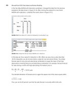
For example, Figure 1-2 shows a list of expense data for a company. The formula in cell C11
uses SUM(C6:C10) to total the January expenses. The idea behind this worksheet is to calculate
a new expense budget number for 2019 as a percentage increase of the actual 2018 total. Cell C3
displays the INCREASE variable (in this case, the increase being used is 3%). The formula that
calculates the 2019 BUDGET number (cell C13 for the month of January) multiplies the 2018
TOTAL by the INCREASE (that is, =C11 * C3).

FIGURE 12 Here is a budget expenses worksheet with two calculations for the January numbers: the total (cell C11) and a
percentage increase for next year (cell C13).

The next step is to calculate the 2018 TOTAL expenses and the 2019 BUDGET figure for
February. You could just type each new formula, but you can copy a cell much more
quickly. Figure 1-3 shows the results when you copy the contents of cell C11 into cell D11. As you
can see, the formula in D11 is =SUM(D6:D10), which means that Excel adjusted the range in
the formula’s function so that only the February expenses are totaled. How did Excel know to do
this? To answer this question, you need to know about Excel’s relative reference format, which I
discuss in the next section.


FIGURE 13 When you copy the January 2018 TOTAL formula to February, Excel automatically adjusts the range reference.

Understanding relative reference format
When you use a cell reference in a formula, Excel looks at the cell address relative to the location of
the formula. For example, suppose that you have the formula =A1 * 2 in cell A3. To Excel, this
formula says, “Multiply the contents of the cell two rows above this one by 2.” This is called
the relative reference format, and it’s the default format for Excel. This means that if you copy this
formula to cell A4, the relative reference is still “Multiply the contents of the cell two rows above
this one by 2,” but the formula changes to =A2 * 2 because A2 is two rows above A4.
Figure 1-4 shows why this format is useful. You had only to copy the formula in cell C11 to cell
D11 and, thanks to relative referencing, everything came out perfectly. To get the expense total
for March, you’d just have to paste the same formula into cell E11. You’ll find that this way of
handling copy operations will save you incredible amounts of time when you’re building
worksheet models.


FIGURE 14 Copying the January 2019 BUDGET formula to February creates a problem.

However, you need to exercise some care when copying or moving formulas. Let’s see what
happens if you return to the budget expense worksheet and try copying the 2019 BUDGET
formula in cell C13 to cell D13. Figure 1-4 shows that the result is 0!
What happened? The formula bar shows the problem: The new formula is =D11 * D3. Cell D11
is the February 2018 TOTAL, and that’s fine, but instead of the INCREASE cell (C3), the formula
refers to a blank cell (D3). Excel treats blank cells as 0, so the formula result is 0. The problem is
the relative reference format. When the formula was copied, Excel assumed that the new
formula should refer to cell D3. To see how you can correct this problem, you need to learn
about another format, the absolute reference format, which I discuss in the next section.
Note
The relative reference format problem doesn’t occur when you move a formula. When you move a
formula, Excel assumes that you want to keep the same cell references.

Understanding absolute reference format
When you refer to a cell in a formula using the absolute reference format, Excel uses the physical
address of the cell. You tell the program that you want to use an absolute reference by placing
dollar signs ($) before the row and column of the cell address. To return to the example in the
preceding section, Excel interprets the formula =$A$1 * 2 as “Multiply the contents of cell A1 by
2.” No matter where you copy or move this formula, the cell reference doesn’t change. The cell
address is said to be anchored.


To fix the budget expense worksheet, you need to anchor the INCREASE variable. To do this,
you first change the January 2016 BUDGET formula in cell C13 to read =C11 * $C$3. After
making this change, copying the formula to the February 2019 BUDGET column gives the new
formula =D11 * $C$3, which produces the correct result.
Caution
Most range names refer to absolute cell references. This means that when you copy a formula that uses a
range name, the copied formula will use the same range name as the original. This might produce errors
in your worksheet.

You also should know that you can enter a cell reference using a mixed-reference format. In this
format, you anchor either the cell’s row (by placing the dollar sign in front of the row address
only—for example, B$6) or its column (by placing the dollar sign in front of the column address
only—for example, $B6).

Tip
You can quickly change the reference format of a cell address by using the F4 key. When editing a
formula, place the cursor to the left of the cell address (or between the row and column values) and then
keep selecting F4. Excel cycles through the various formats. When you see the format you want, select
Enter. If you want to apply the new reference format to multiple cell addresses, select the addresses,
select F4 until you get the format you want, and select Enter.

Copying a formula without adjusting relative references
If you need to copy a formula but don’t want the formula’s relative references to change, follow
these steps:
1.
2.
3.
4.
5.
6.
7.

Select the cell that contains the formula you want to copy.
Place the cursor inside the formula bar.
Use the mouse or keyboard to select the entire formula.
Copy the selected formula.
Select Esc to deactivate the formula bar.
Select the cell in which you want the copy of the formula to appear.

Paste the formula.
Note

Here are two other methods you can use to copy a formula without adjusting its relative cell references:
•

To copy a formula from the cell above, select the lower cell and select Ctrl+’ (apostrophe).

•

Activate the formula bar and type an apostrophe (’) at the beginning of the formula (that is, to the
left of the equal sign) to convert it to text. Select Enter to confirm the edit, copy the cell, and then
paste it in the desired location. Then delete the apostrophe from both the source and destination
cells to convert them back to formulas.


DISPLAYING WORKSHEET FORMULAS
By default, Excel displays in a cell the results of the cell’s formula instead of the formula itself. If you
need to see a formula, you can select the formula’s cell and look at the formula bar. However,
sometimes you’ll want to see all the formulas in a worksheet (such as when you’re troubleshooting
your work).

Displaying all worksheet formulas
To display all the formulas in a worksheet, select Formulas > Show Formulas.

Tip
You can also select Ctrl+` (backquote) to toggle a worksheet between values and formulas.

Displaying a cell’s formula by using FORMULATEXT()
In some cases, rather than showing all the formulas in a sheet, you might prefer to show the

formulas in only a cell or two. For example, if you’re presenting a worksheet to other people, that
sheet might have some formulas you want to show, but it might also have one or more proprietary
formulas that you don’t want your audience to see. In such a case, you can display individual cell
formulas by using the FORMULATEXT() function:
FORMULATEXT(cell)

cell

The address of the cell that contains the formula you want to show

For example, the following formula displays the formula text from cell D9:
=FORMULATEXT(D9)

CONVERTING A FORMULA TO A VALUE
If a cell contains a formula where the value will never change, you can convert the formula to that
value. This speeds large worksheet recalculations and frees memory for your worksheet because
values use much less memory than formulas do. For example, you might have formulas in part of
your worksheet that use values from a previous fiscal year. Because these numbers aren’t likely to
change, you can safely convert the formulas to their values. To do this, follow these steps:
1. Select the cell containing the formula you want to convert.
2. Select F2 to activate in-cell editing. (You can also usually double-click the cell to open it for
editing. If this doesn’t work for you, select File > Options > Advanced, and then select
the Allow Editing Directly In Cells check box.)
3. Select F9. The formula changes to its value.
4. Select Enter or select the Enter button. Excel changes the cell to the value.
You’ll often need to use the result of a formula in several places. If a formula is in cell C5, for
example, you can display its result in other cells by entering =C5 in each of the cells. This is the
best method if you think the formula result might change because, if it does, Excel updates the

other cells automatically. However, if you’re sure that the result won’t change, you can copy only
the value of the formula into the other cells. Use the following procedure to do this:
1.
2.
3.
4.

Select the cell that contains the formula.
Copy the cell.
Select the cell or cells to which you want to copy the value.
Select Home, open the Paste list, and then select Paste Values. Excel pastes the cell’s value
to each cell you selected.

Another method is to copy the cell, paste it into the destination, open the Paste Options list,
and then select Values Only.
Caution
If your worksheet is set to manual calculation (select Formulas > Calculations Options > Manual),
make sure that you update your formulas (by selecting F9) before copying the values of your formulas.

WORKING WITH RANGE NAMES IN FORMULAS
You probably use range names often in your formulas. After all, a cell that contains the
formula =Sales - Expenses is much more comprehensible than one that contains the more
cryptic formula =F12 - F3. The next few sections show you some techniques that make it easier
to use range names in formulas.

Pasting a name into a formula
One way to enter a range name in a formula is to type the name in the formula bar. But what if you
can’t remember the name? Or what if the name is long, and you’ve got a deadline looming? For
these kinds of situations, Excel has several features that enable you to select the name you want
from a list and paste it right into the formula. Start your formula, and when you get to the spot

where you want the name to appear, use any of the following techniques:
•

Select Formulas > Use in Formula and then select the name in the list that appears
(see Figure 1-5).


FIGURE 1-5 Drop down the Use In Formula list and then select the range name you want to
insert into your formula.
•

Select Formulas > Use in Formula > Paste Names (or select F3) to display the Paste Name
dialog box, select the range name you want to use, and then select OK.

•

Type the first letter or two of the range name to display a list of names and functions that
start with those letters, select the name you want, and then select Tab.

Applying names to formulas
If you’ve been using ranges in your formulas and you name those ranges later, Excel doesn’t
automatically apply the new names to the formulas. Instead of substituting the appropriate names
by hand, you can get Excel to do the hard work for you. Follow these steps to apply the new range
names to your existing formulas:
1. Select the range in which you want to apply the names or select a single cell if you want to
apply the names to the entire worksheet.
2. Select Formulas > Define Name > Apply Names. Excel displays the Apply Names dialog
box, shown in Figure 1-6.

FIGURE 1-6 Use the Apply Names dialog box
to select the names you want to apply to your formula ranges.

3. In the Apply Names list, choose the name or names, you want applied from this list.
4. Select the Ignore Relative/Absolute check box to ignore relative and absolute references
when applying names. (See the next section for more information on this option.)
5. Select the Use Row And Column Names check box to tell Excel whether to use the
worksheet’s row and column names when applying names. If you select this check box, you
also can select the Options button to see more choices. (See the section “Using row and
column names when applying names,” later in this chapter, for details.)
6. Select OK to apply the names.

Ignoring relative and absolute references when applying names
If you deselect the Ignore Relative/Absolute option in the Apply Names dialog box, Excel replaces
relative range references only with names that refer to relative references, and it replaces absolute
range references only with names that refer to absolute references. If you leave this option selected,
Excel ignores relative and absolute reference formats when applying names to a formula.
For example, suppose that you have a formula such as =SUM(A1:A10) and a range named Sales
that refers to $A$1:$A$10. With the Ignore Relative/Absolute option deselected, Excel
won’t apply the name Sales to the range in the formula; Sales refers to an absolute range, and
the formula contains a relative range. Unless you think you’ll be moving your formulas around,
you should leave the Ignore Relative/Absolute option selected.

Using row and column names when applying names
For extra clarity in your formulas, leave the Use Row And Column Names check box selected in the
Apply Names dialog box. This option tells Excel to rename all cell references that can be described
as the intersection of a named row and a named column. In Figure 1-7, for example, the range
C6:C10 is named January, and the range C7:E7 is named Rent. This means that cell C7—the
intersection of these two ranges—can be referenced as January Rent.