The effects of rate and amount of reinforcement on the speed of the pacemaker in pigeons’ timing behavior
Bạn đang xem bản rút gọn của tài liệu. Xem và tải ngay bản đầy đủ của tài liệu tại đây (873.45 KB, 7 trang )
Animal Learning & Behavior
1991, 19 (2), 164-170
The effects of rate and amount of reinforcement
on the speed of the pacemaker in
pigeons’ timing behavior
DAVID MACEWEN
Mary Washington College, Fredericksburg, Virginia
and
PETER KILLEEN
Arizona State University, Tempe, Arizona~
The peak-time procedure was used with pigeons to explore assumptions of two models of time
perception: scalar expectancy theory (SET) and behavioral theoryoftiming (BeT). Conditions 1A
and lB varied fixed-interval duration to change rate of reinforcement. Condition 2 varied hopper
duration in order to manipulate arousal level.Condition 3 held constant the interval to be timed
(fixed-interval duration) but varied rate of reinforcement by interspersing trials in which only
the chamber light came on for a duration equal to the fixed interval. Results from Conditions LA,
1B, and 3 show that the speed of the pacemaker (l/r) was directly proportional to the rate of
reinforcement, thus supporting BeT. Manipulations of the hopper duration had no effect on the
timing process.
Recent investigations in animal psychophysics have
shown that animals are extremely accurate at temporal
discrimination (e.g., Church & Deluty, 1977; Dreyfus,
Fetterman, Smith, & Stubbs, 1988; Fetterman & Dreyfus, 1987; Platt & Davis, 1983). Given that organisms
can judge the passage of time, the question remains as
to how they do it. One of the first models of time perception to be developed extensively was that of Treisman
(1963). His model, developed for human time perception,
postulated an internal clock in which a pacemaker emits
pulses at some constant rate, and those pulses increment
a counter. This count is then transferred to a store from
which it may be retrieved by a comparator. If two durations are to be compared, the stored count of the first duration is compared with the current count of the second.
The internal clock model has been adapted to animals’
time perception by Church, Gibbon, and associates (e.g.,
Church, 1984; Gibbon, Church, & Meck, 1984), who
have marshalledmuch empirical support for their account
of the timing process. Gibbon (1977) has offered an elegant set of mathematical models of temporal control,
which he calls scalar expectancy theory (SET). SET assumes that animals form an expectancy of time to reinforcement and that responding is controlled by the ratio
of the instantaneous (moment-to-moment) estimation to
an overall estimation of time to reinforcement. If the time
interval is changed, animals rescale their unit in accorThis research was supported by National Institute of Mental Health
Grant ROl MH43233 to Peter Killeen. We thank J. G. Fetterman for
helpful comments on an earlier version of this manuscript. Requests
for reprints should be addressed to D. MacEwen, Department of Psychology, Mary Washington College, Fredericksburg, VA 22401.
Copyright 1991 Psychonomic Society, Inc.
164
dance with Weber’s law. Time estimates are assumed to
be distributed as a Gaussian function whose variance
should increase as the square of the mean.
Killeen and Fetterman (1988) have proposed an alternative approach, which they call the behavioral theory
of timing (Bet). This theory holds that time judgments are
based on animals’ adjunctive behaviors, which are assumed to serve as discriminative stimuli for the passage
of time. The transitions between different adjunctive behaviors (e.g., from general activity to “terminal” keypecking) are precipitated by pulses from a pacemaker.
Each class of behaviormay be viewed as a manifestation
of an underlying state, with each pulse moving the system from one state to the next. Because the pulses are
assumed to occur with constant probability, transitions between states comprise a Poisson process (Killeen, Hanson, & Osborne, 1978). The equation that embodies this
process is
p[N(t) =n]
=
7
(t/r)’ e
1/Tn!
(1)
where p[N(t) =nj is the probability that the number of
pulses registered by time t equals n and r is the average
time between pulses (see, e.g., Killeen, in press). A key
assumption of the model is that the rateof state transition
(i.e., the rate of the pacemaker, l/r) is directly proportional to the rate of reinforcement in the experimental context. For example, when the rate of reinforcement is doubled the rate ofthe pacemaker is assumed to double. This
assumption is a departure from the previous internal clock
models that assume the rate of the clock to be constant
or, at least, not to change in a systematic way. Moreover,
it provides for a possible empirical test between the BeT
and SET models of time perception.
MANIPULATING PACEMAKER SPEED
Both models have addressed the behavior of animals
under time-based schedules, particularly fixed-interval
(Fl) schedules with the peak procedure (Catania, 1970;
Roberts, 1981). In the peak procedure, the usual Fl contingencies are in effect, with the exception that, on some
trials, food is omitted and the animal is allowed to respond
beyond the time when food would normally be delivered.
When response rates are plotted for successive segments
of the food omission trials, the resulting function is approximately normal, with the peak (mode) at about the
point when food would normally be delivered. Both
models view this function to be the result of a timing
process but assume quite different things about it.
BeT assumes that the animal advances through several
interim behavioral states according to a Poisson process
until it enters a terminal state of, say, keypecking. The
normal distribution of pecking is the result of averaging
many terminal state entries and exits. The Fl scallop is
the left limb of the normal distribution reflecting entries
into the pecking state. The right limb, reflecting exits from
the pecking state, is measurable on trials during which
food is omitted. The rate at which the animal advances
to the terminal state and the amount of time it resides in
that state is assumed to be determined by the rate of reinforcement. The assumption of an underlying Poisson
process results in a mean of (n +1 )r and a variance of
2
(n + l)r for the distribution in the simplest case (i.e., the
animal stays in each state until one additional pulse is
registered).
SET assumes that the response-rate function reflects the
animal’s estimates of the Fl as an expectancy of time to
reinforcement. These estimates are assumed to be distributed as the difference of two Gaussian distribution
functions. (Roberts, 1981, fit his data to a Gaussian distribution, but SET specifies the difference of two cumulative Gaussian distributions; see Equation 2 below.) The
animal begins responding only when the ratio of the local or momentary expected time to reinforcement to the
overall expected time to reinforcement exceeds some
threshold value (Gibbon, 1977). Both the mean and the
standard deviation of the Gaussian functions are assumed
to be proportional to the interval being timed; hence, the
coefficient of variation (a//2) should remain constant when
the Fl duration is changed. The invariance of this
parameter is taken as a measure of sensitivity to time comparable to the Weber fraction.
The present experiment utilized the peak procedure to
assess some of the assumptions about the timing process
made by BeT and to compare the results with assumptions from SET. The first manipulation varied Fl duration as a way of changing rate of reinforcement. BeT assumes that the response-rate function should be described
by a Poisson process and the rate of the pacemaker (lIr)
should be directly proportional to rate of reinforcement.
That is, the ratio of the values of r at two Fl durations
should equal the ratio of the values of the time to reinforcement for those same two Fl durations.
165
A second manipulation examined the possible role of
arousal on r. Killeen, Hanson, and Osborne (1978) demonstrated that a single presentation of food led to an increase in arousal level as measured by general activity.
They reported that different hopper durations led to different levels of general activity, but that, in all cases, activity decreased over time at the same rate. It is possible that
the rate of the pacemaker is a direct function of arousal
level and that changing rate of reinforcement is just one
way of changing arousal. Alternatively, both the rate of
the pacemaker and the arousal level are functions of rate
of reinforcement, and other variables (e.g., amount) may
affect one but not the other. Although SET has a motivational parameter, H, that is assumed to vary with the
amount of (or access to) the reinforcer, H gets canceled
out of the expectancy ratio. SET therefore predicts that
varying arousal or motivational level should have no effect on the timing process. In an attempt to change arousal
level and measure the effect on the rate of the pacemaker,
amount of food (hopper duration) was varied.
A third manipulation extended our investigation of the
role of reinforcement rate on r. When the rate of reinforcement is decreased by doubling Fl duration, the interval to be estimated is doubled, and the expectation of
time to reinforcement should also double. SET and BeT
make the same predictions in this case. Rate of reinforcement was therefore manipulated by holding Fl duration
(the interval to be estimated) constant but instituting blank
trials between regular trials. These blank trials omitted
keylight and reinforcement and proportionally increased
the interreinforcement interval. Since the keylight was off
and no food was ever presented during chamber-light-only
presentations, SET would presumably hold that the timing process was not operative and no expectancy was
present. Thus, r could be manipulated while holding constant expectation to reinforcement. Because expectancy
of time to reinforcement does not change in this manipulation, SET predicts no changes in parameter values in
its equations. Under the two different rates of reinforcement (chamber-light condition vs. no-chamber-light condition), BeT predicts that the value of r should vary and
the ratio of the values of r should equal the ratio of the
values of the two different interreinforcement intervals.
Method
Subjects
Four Silver King pigeons were maintained at 80% (±10 g) of
their free-feeding weights. All animals had previous experience keypecking for food under various schedules of reinforcement.
Apparatus
A standard two-key Lehigh Valley Electronics pigeon chamber
served as the experimental space. The left key remained dark and
inoperative throughout the experiment. The right key was 22 cm
above the chamber floor and could be illuminated by a green light.
Key switch closure required a force of 0. lN. Chamber illumination was provided by a miniature lamp centered on the front wall
32 cm above the floor. Mixed grain was occasionally presented
166
MAcEWEN AND KILLEEN
through an
opening centered on the front wall, 5 cm square and
10 cm above the chamber floor. White noise was continuously
presented to mask extraneous sounds. A ventilation fan provided
fresh air and additional masking. A microcomputer controlled the
experiment and recorded data.
Procedure
All birds were exposed to an autoshaping program for two sessions and then switched to Fl schedules of reinforcement. The Fl
duration was increased over the next few sessions until all birds
were responding under a Fl 30-sec requirement. During the fixed
interval, the key was illuminated with a green light and the chamber was illuminated by the white chamber light. A key switch closure
following the Fl 30 sec turned off the keylight and the chamber
light and provided 3-sec access to mixed grain. The 3-sec feed duration was timed from the point when the bird broke a photobeam
with its head upon entering the feeder opening. Following food
presentation, all lights remained off for a 15-sec intertrial interval
(ITT). This sequence of events was repeated for 60 grain presentations (trials). All subjects showed stable responding under the Fl 30sec schedule after 10 consecutive days. Stability was assessed by
visual inspection of a plot of the latencies from keylight onset until
the third keypeck.
After the 10th session, 2 subjects were switched to Fl 14-sec
(Birds 14 and 41), 2 subjects were switched to Fl 35-sec (Birds
36 and 37), and apeak procedure was instituted. For 12 of the 60
trials, the contingency between a keypeck and grain delivery was
not in effect; instead, the trial continued for twice the usual Fl duration. Thereafter, the trial terminated with a probability of 0.15
every 2 sec (for the Fl 14 see) or every 5 sec (for the Fl 35 see).
This continued for a maximum of six possible additional extensions.
Whenever the trial was terminated, no grain was delivered and all
lights went off for the 15-sec ITI. If the Fl is x, with bin size of
x/7, the average duration of a peak trial is 3x. The 12 peak trials
were randomly presented each session.
Fl 14-sec schedule and birds 36 and 37 were switched to an Fl 35sec schedule, with the chamber-light manipulation still in effect.
These contingencies were again maintainedfor 25 consecutive days.
Dependent Measures
Rates of keypecking during peak trials were recorded for each
of the 20 possible response bins. The bimeans (see Killeen, 1985)
over the last 10 days of each experimental phase were obtained for
each response bin. In addition, latencies to the third keypeck for
each trial were collected for each session in each phase. No data
were recorded during ITI, food presentations, or chamber-lightonly trials. Only data from peak trials were used in the analysis.
Inferred Measures
The parameters j~and a were inferred by fitting Equations 2 and
5 to the data choosing values that minimized the sum of squared
deviations. The parameters r and n were then inferred from ~cand
a by solving Equations 3 and 4. In all cases, parameters were derived from averaged data ofthe subjects that experienced the same
contingencies.
RESULTS
Condition 1
Figure 1 presents response rates for each of the first
13 bins during peak trials of Conditions 1A and lB. Data
points (squares) represent the bimean of response rates
for the last 10 sessions averaged over the 4 birds. The
top panel shows data from the Fl 14-sec condition (t =
14 sec); the bottom panel shows data from the Fl 35-sec
condition (t = 35 sec). In both cases, the data increase
Condition 1A
Two birds (Birds 14 and 41) were trained under a peak procedure using an Fl 14-sec schedule; the other 2 birds (Birds 36 and
37) were similarly trained using an Fl 35-sec schedule. The criterion for stable responding was the same as mentioned above. All
birds were trained for a minimum of 25 days.
a ~
125
C
E
U)
a
U)
C
0
U)
a
Condition 2
Duration of food was varied. Birds 14 and 37 were switched to
1.5-sec food access and Birds 41 and 36 were switched to 7-sec
food access. After 25 days, food-access times were reversed: Birds
14 and 37 received 7-sec access to food and Birds 41 and 36 received
1.5-sec access to food for an additional 25 days.
Condition lB
All birds were returned to conditions with 3-sec access to food
for 10 sessions. The Fl durations were then switched for the birds.
Birds 14 and 41 were switched to an Fl 35-sec schedule; Birds 36
and 37 were switched to an Fl 14-sec schedule. All birds continued
to receive 12 randomly presented peak trials each session. All birds
showed stable responding after 25 daily sessions.
Condition 3
The contingencies of Condition lB remained in effect during Condition 3, except that the chamber light cameon for a duration equal
to the Fl after each ITI. During this time, the keylight was off,
the key switch was inoperative, and no food was ever presented.
Following the offset of the chamber light, a 15-sec ITI was again
in effect. Peak and regular Fl trials alternated with chamber-lightonly exposures throughout the session. These contingencies were
maintained for 25 days. Birds 14 and 41 were then switched to an
a
U)
25
0
0
10
15
20
25
Time (see)
-~
E
100
U)
75
C
0
0.
~
U)
50
25
40
Time (sec)
Figure 1. Response rates (pecks per minute) for each of the first
13 bins during peak trials in Conditions 1A and lB. Each data point
represents the bimean of response rates for the last 10 sessions averaged over the 4 birds. The curves are derived from Equations 2 and 5.
MANIPULATING PACEMAKER SPEED
smoothly to a maximum close to the expected time ofreinforcement and then decrease to a minimum at twice the
training value. Thereafter, the data for the remaining bins
(not shown) increase erratically to about one fourth of the
peak rate. Church, Miller, Gibbon, and Meek (1988) reported a similar delayed increase for rats and, in a careful series of experiments, demonstrated that it disappeared
when several factors confounding the basic timing task
were minimized.
The theoretical responserate (R1) is proportional to the
difference of two normal distributions:
R1
=
k[~(J4l,a1)—~(Jt2,az)],
(2)
where 4(ji,a) is a cumulative normal distribution of mean
and standard deviation a, and k is a constant ofproportionality.
Both SET and BeT employ this equation to account for
various types of data (Gibbon, 1977). BeT assumes that
the underlying system is a Poisson process—an assumption that we treat as a “default” assumption, because it
provides one of the more obvious and tractable models.
A more reasonable assumption might be that the pacemaker is somewhat more accurate and the accumulator
is somewhat less than perfect. This would also lead to
Equation 2 as a convenient approximation, but would
stipulate different relationships among the parameters of
the distributions (see the Appendix of Killeen & Fetterman, 1988).
Under the Poisson assumption, the mean and variance
of the normal distribution governing entry into the response state are
~t
=
(n+l)r
13\
and
a2
=
(n+1)r2,
(4)
where n is the number of pulses from the pacemaker be-
fore pecking begins and r is the period of the pacemaker.
The mean and variance of the distribution governing exit
from the response state are governed by similar equations.
A theoretical assumption reduces the number of free
parameters: According to BeT, r must remain invariant
within the experimental context, and so the calculations
for both entry and exit share the same values of r.
How long will the animals stay in the response state?
That is an empirical question, and the data, as viewed
through this model, permit anywhere between one and
three pulses before the animal exits from the response
state. However, changes in the assumed dwell time had
very little effect on the goodness of fit; so, for simplicity, we have assumed that residence time is uniformly a
single pulse and have analyzed all the data according to
that convention. Thus, in calculating the parameters of
the normal distributions for exit, we use n+ 1 and r.
Equation 2 gives the probability ofbeing in the response
state correlated with pecking, but it does not tell us the
response rate while in that state; it is not immediately obvious how to translate probability into rate. The problem
arises because responses are not instantaneous. Each time
167
a response is made, it reduces the time available during
which other responses might be emitted. If responses are
attempted randomly in time at a “theoretical” rate of R1,
and each response blocks the emission of other responses
for (ô) seconds, then the measured response rate (Rm) will
be approximately
Rm
=
R1/(1 +6R1)
(5)
(Bharucha-Reid, 1960, Equation 51; Killeen, 1981, Equation 19). At low rates of responding and for small values
of b, Rm = R1 however, at response rates that are high
relative to the maximum rate, this ceiling effect will cause
a concave departure from linearity toward an asymptotic
rate of ho.
The above mapping was used to get from the probabilistic predictions of Equation 2 to actual response rates. The
equations introduce two new parameters: the rate of responding given that the animal is in the response state correlated with pecking (Rm) and the maximum sustainable
response rate (1/0). Although a model such as this was
necessary to accommodate these data, the fit is not perfect (as can be seen in the top panel of Figures 1 and 4),
where the rates came against a firmer ceiling than that
pictured by Equation 5.
Values for the key parameters from Equations 2-5 are
presented in Table 1 for the two Fl values of Conditions
1A and lB. In addition, Table 1 shows the proportion of
variance accounted for by the model. Figure 2 presents
the recovered values of r across reinforcement conditions
for each bird (Birds 14, 41, 36, and 37), as well as a function fit to the averaged data.
A key assumption in BeT is that the value of r, the
period of the pacemaker, should be proportional to the
time between reinforcements. All birds showed an increase in the value of r when the period of reinforcement
was decreased by shifting from Fl 14 sec to Fl 35 sec.
The slope of the line fit to the averaged data was reliably
greater than zero [t(3) = 8.09, p < .01]. Under this peak
procedure, the ratio of values for the average time between reinforcers under the two conditions was 2.5 and
the ratio of the two Fl values was also 2.5. The ratio of
r under Fl 35 to r under Fl 14 was found to be 2.7, close
to the predicted value of 2.5. The slope of the regression
line fit to values of r under each H condition was not reliably different from 2.5 [t(3) = 1.55, n.s.], supporting the
notion that r is directly proportional to the time between
Table 1
Key Parameters of Equations 2—5 and Proportion of Variance
Accounted for by the Model for Conditions 1A and lB
Subject
n
r (14 see)
r (35 see)
ô (msec)
PVA
14
8
1.4
3.6
375
.972
41
8
1.3
3.5
240
.985
36
7
1.6
4.3
480
.916
37
6
1.6
4.4
480
.955
Average
7
1.5
4.1
375
.957
Note—PVA = proportion of variance that was accounted for by the
model.
168
MAcEWEN AND KILLEEN
amount (hopper duration) had no effect on r. Peak response rates for the 1.5-, 3.0-, and 7.0-sec durations were
144, 122, and 131 responses per minute for the Fl 14-sec
condition and 101, 108, and 89 responses per minute for
the Fl 35-sec condition.
5.
Conditio ,,,1~,,,)
1
4
Q
aU)
3
:2
U)
I-
0
10
20
30
40
Ft Value (see)
Figure 2. The recovered values of r across reinforcement conditions of Fl 14 sec and Fl 35 sec for each of the 4 birds (Birds 14,
41, 36, and 37) from Conditions 1A and lB. The regression line
through the average data shows that r is proportional to the time
between reinforcements.
Table 2
Key Parameters of Equations 2—5 and Proportion o f Variance
Accounted for by the Model for Condition 2
Amount
n
r (see)
ô (msec)
PVA
1.5
3.0
7.0
1.5
3.0
7.0
Note—PVA
model.
7
7
7
=
Fl 14 sec
1.5
1.5
1.6
375
375
375
.964
.972
.964
Fl 35 sec
7
3.9
315
.962
7
4.1
315
.971
7
3.9
315
.989
proportion of variance that was accounted for by the
reinforcements. The use of a fixed intertrial interval might
have made it possible for the pigeons to ignore the stimuli
and time each trial from the end of the previous trial. That
this did not happen is shown by the data in Figure 1, which
rise from an origin of 0 sec at the beginning of the interval. The count started when the keylight came on. It is
nonetheless possible that the ITI added to the timebase
for reinforcement and thus affected the speed of the
pacemaker. Because we did not differentially manipulate
ITI in this experiment, however, we cannot comment on
this possibility.
Condition 2
Table 2 presents key parameters from Equations 2-5
for each of the two Fl durations at each hopper duration
(1.7, 3.0, and 7.0 see), as well as the proportion ofvariance accounted for by the model. The data for the Fl 14sec schedule are averaged over Birds 14 and 41, and those
for the H 35-sec schedule are averaged over Birds 36 and
37. Data for the 3.0-see hopper duration were taken from
Condition lA and averaged over all 4 subjects.
Figure 3 shows the values of r, the period of the pacemaker, when amount of reinforcement was varied. The
solid bars correspond to the H 14-sec condition; the stippled bars correspond to the H 35-sec condition. Food
Condition 3
Table 3 presents key parameters of Equations 2-5 under the standard peak procedure described earlier and
when sessions were extended with trials in which the
chamber light was kept on for a duration equal to the Fl
schedule in effect. The intent of this manipulation was
to decrease the period of reinforcement while holding the
duration to be timed constant. The data for the Fl 14-sec
schedule are averaged over Birds 41 and 37, and those
for the Fl 35-sec schedule are averaged over Birds 14 and
36. Proportion of variance accounted for by the model
is also presented in Table 3. The period of the pacemaker
was clearly decreased by the extended time between reinforcements. Table 3 shows that when the values of r were
held at those obtained from the standard peak procedure
of Conditions lA and 1B, proportion of variance accounted
for decreased considerably (even though n was let to float
to the value that optimized goodness of fit). We cannot
presume constancy of the pacemaker without giving up
10 points of accuracy in fitting the data. Letting r assume
the value that maximizes goodness of fit, Table 3 shows
that, for the Fl 14-sec schedule, rdecreased from 1.5 sec
in the standard condition to 2.4 sec in the extended condition; for the Fl 35-sec schedule, r decreased from
4.0 sec in the standard condition to 6.8 sec in the extended
condition.
The average time (T) between reinforcers was proportional to the Fl value; the ratio of the values of T under
the standard and chamber-light-extended conditions was
1.71. The slope of the regression of the data was reliably
greater than zero [t(3) = 4.63, p < .01] and not reliably
different from 1.71 [t(3) = .67, n.s.]. Thus, the hypothesis that the period of the pacemaker is directly proportional to the time between reinforcementswas again supported.
U
Condition 2
F114-sec
l~F135-sec
S
M
L
Amount of Food (see)
Figure 3. Bars represent average values of r when amount of reinforcement (hopper duration) was varied. Solid bars represent the
Fl 14-sec schedule; stippled bars represent the Fl 35-sec schedule.
MANIPULATING PACEMAKER SPEED
Table 3
Key Parameters of Equations 2—5 and Proportion of Variance
Accounted for by the Model for Condition 3
Condition
n
r (see)
ó (msec)
PVA
Standard
Extended
Extended
7
7
4
Fl 14 sec
1.5
1.5*
2.4
.977
.819
.942
315
315
315
Fl 35 sec
Standard
7
4.0
375
.984
Extended
6
4.0*
375
.838
.931
Extended
3
6.8
375
Note—PVA = proportion of variance that was accounted for by the
model.
*Values were held at the standard value and the fit was otherwise optimized.
Figure 4 shows response rates (pecks per minute) for
each ofthe first 13 bins during peak trials of Conditions lA
and lB (filled squares) and Condition 3 (open squares). The
top panel shows the data from the Fl 14-see schedule; the
bottom panel shows the data from the H 35-sec schedule.
Data points are bimeans of response rates for the last 10
sessions averaged over the 2 birds in each condition. As
before, the fitted curves are derived from the difference
between two normal distributions. Although in both cases
C
E
U)
a
U)
C
0
0.
U)
a
a
U)
Time (see)
Ft 35-sec
C
E
U)
aU)
C
0
0.
U)
a
a
U)
0
20
40
60
Time (see)
Figure 4. Response rates (pecks per minute) for each of the first
13 bins during peak trials of Condition lA and lB (filled squares)
and for peak trials of Condition 3 where interreinforcement time
was extended (open squares). The top panel shows the data from
the Ft 14-sec schedule; the bottom panel shows the data from the
F! 35-sec schedule. Data points are bimeans of response rates for
the last 10 sessions averaged over the 2 birds in each condition.
Smooth curves are functions fit to the data from Equations 2 and 5.
169
the functions approximate the data, the approximation is
better for the peak trials of Conditions 1 A and lB than
for peak trials from the extended interreinforcement duration of Condition 3. The variance of the distribution increased under this manipulation, as expected, although the
mean of the distributions either did not change (H 14 see)
or decreased. Equations 3 and 4 show us that changes in
r can be compensated for by changes in n to keep either
2
~t or a constant, but no compensatory changes can keep
both constant. Under the Fl 14-sec schedule, the pigeons
kept ~a constant at the price of an increase in a2. Under
the Fl 35-see schedule, a2 increased and ~i decreased.
DISCUSSION
Conditions 1 A and lB replicated the “peak-time” effect in pigeons and showed that the scalar timing demonstrated was consistent with predicted variations in the speed
of the pacemaker. The period of the pacemaker (lIT) was
found to be directly proportional to the period of reinforcement in the experimental setting. By themselves,however, the results of Conditions 1A and lB do not differentiate between the assumptions of SET and BeT. Because
the period of reinforcement was manipulated by changes
in Fl schedule duration, one could argue that either the
period of the pacemaker or the expectation to reinforcement was the causal factor. In Condition 2, changes in
amount of reinforcement had no effect on the parameters
of the distributions fit to the data. This finding is consistent with the SET model, in which the motivational
parameters cancel out of the expectancy ratios underlying timing performance. We had expected to see some
effect of amount in Condition 2, since changes in arousal
due to footshock affect pacemaker speed (Meck, 1983).
However, in a recent review of the literature concerning
the effects of magnitude of reinforcement, Bonem and
Crossman (1988) concluded that “the question of whether
magnitude of reinforcement is or is not effective remains
open to debate” (p. 359). Some studies have even found
an inverse relation between amount of reinforcement and
response rate (Staddon, 1970). Staddon explains these
results as being due to a postreinforcement inhibitory effect similar to that found with the omission procedure.
Notice that in the present experiment there was no systematic change in peak rate as amount of food was
varied—if anything, it tended to decrease for the largest
amount. Although this 5-to- 1 change in amount of food
had no systematic effect on response rate, the 2.5-to-l
change in reinforcement rate between the 14- and the 35sec schedules did have a systematic effect on peak rate
in the expected direction. Thus, there is no evidence that
manipulation of amount of food affected arousal level (as
inferred from response rate). It is also certainly apparent
in Figure 3 that manipulation of amount of food had no
effect on the speed of the pacemaker. Beyond that, it is
not clear in the present experiment whether (1) arousal
level does affect pacemaker speed, but difference in hopper time did not generate differences in arousal, or
170
MAcEWEN AND KILLEEN
(2) arousal level does not determine pacemaker speed,
even though it may be affected by some of the same variables that affect pacemaker speed.
Condition 3 showed that extending the interreinforcement interval without changing the interval to be estimated
(Fl duration) affected the speed of the pacemaker. These
results are similar to those of Holder and S. Roberts
(1985) and S. Roberts and Holder (1985), who used a
peak procedure and found that stimulus durations were
not timed by the rats unless the signal was directly paired
with primary reinforcement. In addition, W. A. Roberts,
Cheng, and Cohen (1989) found that when pigeons were
tested with time-outs midway through a peak trial, they
did not continue timing during the time-out, but reset the
timing mechanism to 0 sec. These procedures, using both
rats and pigeons, are analogous to our chamber-light-only
presentations, which were never directly paired with reinforcement and were always followed by an ITI. The results of Condition 3 are consistent with the assumptions
and predictions of the BeT model. Since the interval to
be timed is not changed in Condition 3, the assumptions
from SET predict that scalar timing should not be affected.
However, we can see in Figure 4 that the variance increased and the pacemaker slowed.
Taken together, the results from all three conditions do
not unequivocally rule out either model. In the standard
peak procedure using FT schedules, both models make the
same predictions. The results from Condition 2 follow
from SET, since the motivational parameter, H, plays no
role in the final expectancy ratio. The results clarify some
of the causal factors in BeT: they teach us that amount
of reinforcement may have no effect on the pacemaker
speed for pigeons. However, the results do not rule out
the hypothesis that pacemaker speed may be controlled
by arousal level, because there is no evidence from response rate that arousal level was changed by the different amounts of food. The results of Condition 3 favor the
BeT model. One central assumption of BeT is that the rate
of the pacemaker is directly proportional to the rate of
reinforcement. When the interval to be timed is held constant while rate of reinforcement is varied, BeT predicts
that the animal’s clock will also vary. SET has no means
to accommodate the findings of Condition 3, since expectation to reinforcement does not change and clock speed
is assumed to not vary. Neither model, however, would
take pride of ownership in the mediocre fit of Equation 2
to the data from the extended trials of Condition 3.
REFERENCES
Schoenfeld (Ed.), The theory of reinforcement schedules (pp. 1-42).
New York: Appleton-Century-Crofts.
CHURCH, R. M. (1984). Properties of the internal clock. In J. Gibbon
& L. Allan (Eds.), Annals of the New York Academy of Sciences:
Vol. 423. Thning and time perception (pp. 566-582). New York: New
York Academy of Sciences.
CHURCH, R. M., & DELUTY, M. Z. (1977). Bisection of temporal intervals. Journal of Experimental Psychology: Animal Behavior
Processes, 3, 216-228.
CHURCH, R. M., MILLER, K. D., GIBBON, J., & MECK, W. (1988,
November). Symmetrical and caynvnetrical sourcesof variance in temporal generalization. Paper presented at the annual meeting of the
Psychonomic Society, Chicago.
DREYFUS, L. R., FETTERMAN, J. G., SMITH, L. D., & STUBBS, D. A.
(1988). Journal of Experimental Psychology: Animal Behavior
Processes, 14, 349-367.
FETTERMAN, J. G., & DREYFUs, L. R. (1987). Duration comparison
and the perception of time. In M. L. Commons, J. E. Mazur,J. A.
Nevin, & H. Rachlin (Eds.), Quantitative analysis of behavior: Vol. 5.
Reinforcer value— The effect of delay and intervening events (p. 27).
Hillsdale, NJ: Erlbaum.
GIBBON, J. (1977). Scalar expectancy theory and Weber’s law in animal
timing. Psychological Review, 84, 279-325.
GIBBON, J., CHURCH, R. M., & MECK, W. H. (1984). Scalar timing
in memory. In J. Gibbon & L. Allan (Eds.), Annals of the New York
Academy of Sciences: Vol. 423. liming and time perception (pp. 5277). New York: Appleton-Century-Crofts.
HOLDER, M., & ROBERTS, S. (1985). Comparison of timing and classical conditioning. Journal of Experimental Psychology: Animal Behavior Processes, 11, 172-193.
KILLEEN, P. R. (1981). Averaging theory. In C. M. Bradshaw,
E. Szabadi, & C. F. Lowe (Eds.), Quantification of steady-state operant behaviour (pp. 21-34). New York: Elsevier.
KILLEEN, P. R. (1985). The bimean: A measure of central tendency
that accommodates outliers. Behavior Research Methods, Instruments,
& Computers, 17, 526-528.
KILLEEN, P. R. (in press). Behavior’s time. In G. H. Bower (Ed.), The
psychology of learning and motivation: Advances in research and theory (Vol. 27).
Killeen, P. R., & Fetterman, J. G. (1988). A behavioral theory oftiming. Psychological Review, 95, 274-295.
Killeen, P. R., Hanson, S. J., & Osborne, S. R. (1978). Arousal: Its
genesis and manifestation as response rate. Psychalogical Review, 85,
571-581.
MECK, W. H. (1983). Selective adjustment ofthe speed ofinternal clock
and memory processes. Journal ofExperimental Psychology: Animal
Behavior Processes, 9, 171-201.
PLATT, F. R., & DAVIS, E. R. (1983). Bisection of temporal intervals
by pigeons. Journal of Experimental Psychology: Animal Behavior
Processes, 9, 160-170.
ROBERTS, 5. (1981). Isolation of an internal clock. Journal of Experimental Psychology: Animal Behavior Processes, 7, 242-268.
ROBERTS, S., & HOLDER, M. D. (1985). Effects ofclassical conditioning on an internal clock. Journal of Experimental Psychology: Animal
Behavior Processes, 11, 194-214.
ROBERTS, W. A., CHENG, K., & COHEN, J. S. (1989). Timing light
and tone signals in pigeons. Journal of Experimental Psychology:
Animal Behavior Processes, 15, 23-35.
STADDON, J. E. R. (1970). Effects of reinforcement duration on fixedinterval responding. Journal of the Experimental Analysis of Behavior,
13, 1-31.
A. T. (1960). Elements of the theory of Markov
processes and their applications. New York: McGraw-Hill.
BONEM, M., & CROSSMAN, E. K. (1988). Elucidating the effects of reinforcement magnitude. Psychological Bulletin, 104, 348-362.
CATANIA, A. C. (1970). Reinforcement schedules and psychophysical
judgments: A study ofsome temporal properties ofbehavior. In W. N.
BHARUCHA-REID,
M. (1963). Temporal discrimination and the indifference
interval: Implications for a model of the “internal clock.” Psychological Monographs, 77(Whole No. 756).
TREISMAN,
(Manuscript received August 3, 1989;
revision accepted for publication December 6, 1990.)