Application of directional derivative method to determine boundary of magnetic sources by total magnetic anomalies VJES 39

Vietnam Journal of Earth Sciences, 39(4), 360-375, DOI: 10.15625/0866-7187/39/4/10731
Vietnam Academy of Science and Technology

(VAST)

Vietnam Journal of Earth Sciences
/>
Application of directional derivative method to determine
boundary of magnetic sources by total magnetic anomalies
Nguyen Thi Thu Hang1, Do Duc Thanh*1, Le Huy Minh 2
1

Hanoi University of Science (VNU)

2

Institute of Geophysics (VAST)

Received 27 May 2017. Accepted 01 September 2017
ABSTRACT
This paper presents the Directional Derivative method to determine location and boundaries of the magnetic directional structure sources through a new function DG (Directional Gradient - DG). Algorithm and computer program
are made a code by Matlab language to attempt to calculate on 3D models in the compare with Horizontal derivative
method (HG). A new function DG also applied to determine the boundary of magnetic sources by the total magnetic
anomalies of Tuan Giao region. The result shows that with the application of new function DG, the boundaries of
magnetic sources are exactly defined although they have a directional structure and small horizontal size. Moreover,
because it does not depend on directions of magnetization, so in the computation, the transformation of the magnetic
field to the pole can ignore, thus, reduce transient error. Alternatively, with the application of new function DG, the
interferences in case the sources distributed close together are overcome. This usefulness affirms the possibility of
application of the this method in the analysis and interpretation of magnetic data in Vietnam.
Keywords: Magnetic anomaly; Magnetized prism; Horizontal Gradient; Directional Gradient; Tuan Giao.
©2017 Vietnam Academy of Science and Technology

1. Introduction*
In magnetic exploration, the quantitative
interpretation or the solution of the inverse
problem to determine the location, shape,
depth, magnetization of geological objects
causing observed anomalies always plays an
important role. In recent years, in Vietnam,
many modern methods for determining the location of geological sources based on total
magnetic anomalies ΔTa have been studied
and applied such as the method of determining maximum horizontal gradient vector field
                                                            
*

Corresponding author, Email:

360

(Le Huy Minh et al., 2001; Le Huy Minh et
al., 2002), the method of calculating vertical
derivative and its maximum horizontal gradient vector (Vo Thanh Son et al., 2005), the
method of analytic signals (Vo Thanh Son et
al., 2005; Vo Thanh Son et al., 2007). The research results show that besides the advantages, these methods have many limitations in overcoming the problem of interference in case the actual conditions are complex
and the differentiation of the sources is not
clear. On the other hand, the studies also show
that in most methods, the accuracy of analytical results depends on the isometry and
magnetization inclination of the anomaly-


Nguyen Thi Thu Hang, et al./Vietnam Journal of Earth Sciences 39 (2017)

generating object. It makes the analysis, processing, and interpretation of magnetic data
by these methods more complicated because
they must be combined with the calculation
programs for reduction to the pole. In addition, this intermediate step will result in significant errors in the analysis, especially in
case the study area is located in a low-latitude
region. Based on this fact, in this article, we
have studied and proposed the application of
directional gradient (DG) in combination with
the determination of the maximum of DG
function (|DGmax|) according to the algorithm
of Blakely and Simpson (1986) in order to define the boundary of banded geological objects which extend in one direction and have
different magnetic properties in the Earth’s
crust. The method is implemented by a program written in the Matlab language which
has been tested on 3D models in comparison
with the method of calculating maximum horizontal gradient vector field (HG). The DG
function is also used to interpret the aeromagnetic anomaly map in Tuan Giao area, thereby
evaluating the effectiveness of the presented
method.
2. Methodology
2.1. Horizontal derivative
Suppose f(x, y) is a smoothly-varying scalar quantity measured on a horizontal plane.
The horizontal derivatives of f(x, y) are easily
evaluated by using the finite difference method and the measured values of f(x, y). If fij,
with i=1, 2,…, j=1, 2,… are the measured
values of f(x, y) on a regular grid with the
steps x and y, the horizontal derivatives of
f(x, y) at the point (i, j) is approximated by:

df ( x, y ) f i 1, j  f i 1, j


2 x
dx
df ( x, y ) fi , j 1  f1, j 1
 

dy
2 y

(1)

The horizontal derivatives are also easily
implemented in the frequency domain. Ac-

cording to difference theory, the Fourier transform of nth-order horizontal derivatives of f(x,
y) is defined as follows:
dn f 
n
F  n    ik x  F  f 
 dx 
(2)
n
n
d f 
F  n   ik y F  f 
 dy 

 

Thus, in the frequency domain, the calculation of horizontal derivative of a potential

field measured on a horizontal plane can be
defined as a three-step filtering operator: Fourier transform of potential field, multiplication
by the corresponding filters (ikx)n and (iky)n,
and then inverse Fourier transformation of obtained products.
2.2. Directional derivative
The directional derivative denoted as

Dsˆ f is the rate of change of f(x,y) at the point
(x 0 , y 0 ) in the direction of unit vector sˆ . It is

a vector form of the usual derivative and can
be defined as:
 s
f ( x  ah, y  bh)  f ( x, y) (3)
Dsˆ f ( x, y)   f .   lim

h
0
s
h

Where  is the nabla operator and sˆ is
the unit vector in the Cartesian coordinate system. In the horizontal plane, with sˆ  ( s x , s y ) ,



we have: sˆ 
thus

Dsˆ f ( x, y ) 

sx2  s y2 =1

f ( x, y )
f ( x, y )
sy
sx 
x
y

(4)
If sˆ makes an angle  with the positive
side
of
the
Ox
axis,
then
we
ˆ



s
(
c
os
,sin
)
. Therefore, the derivahave

tive of f(x, y) in the direction of the vector sˆ
is:
f ( x, y )
f  x, y 
cos 
sin  (5)
Dsˆ f ( x, y ) 
y
x
If f(x, y) is the function of total magnetic
anomalies ΔT(x, y) caused by an object whose
extending direction makes an angle α with the
361


Vietnam Journal of Earth Sciences, 39(4), 360-375 

Oy axis, then according to the above definition, at the point M(x, y) on the horizontal
plane, the derivative of ΔT(x, y) in the
direction of the vector sˆ , which is
perpendicular to the structural direction of the
source, is defined as follows:
T
T
(6)
Dsˆ T 
cos  
sin 
x
y

In numerical calculation, the values of the
magnetic field are observed on a regular grid,
the DG function representing derivative values on the horizontal plane at the point (i, j) in
the direction sˆ (Figure 1) is defined by the
formula:

ed by a quadratic polynomial. Then, the magnetic field interpolated at the point M is defined by:
 TM (x, y) = a(x-x0)2 + b(x-x0)(y-y0) +
(8)
c(y-y0)2+ d(x-x0) + e(y-y0) + f
where (x0, y0) are the coordinates of the point
(i+1,j+1) selected as the origin, (x,y) are the
coordinates of M, and the coefficients of expansion a, b, c, d, e, f are selected in such a
way that:


N

Pk [ Tqs ( k ) - T (k ) ]2 = min

(9)
       
where Tqs ( k ) is the value of magnetic field
k 1

observed at the kth point among N observation
points within the radius R. Pk is the weighting
function, defined as follows:

 R d2 

Pk   2 k 
 dk  

Figure 1. The sˆ directional gradient of total magnetic
anomaly field at observation point (i,j)

DG DsˆTi, j 

TM  TN
with d = |MN| (7)
d

In case M and N do not coincide with the
grid cells, we use the interpolation method to
find the values ∆TM and ∆TN. In order to find
∆TM, we perform the following steps:
Using the algorithm to select the grid cell
closest to M as the origin. In this case, it is the
point (i+1, j+1).
The value of ∆TM is determined by the
method of least squares. According to this
method, the magnetic field around the origin,
namely the point (i+1, j+1), within the radius
R, containing N observed values is represent362



(10)

where dk is the distance from the origin to the

kth point;  and  are the coefficients.
The determination of the value of magnetic
field ∆TN at the point N is similarly carried
out. In this case, the point selected as the
origin for the interpolation is the point (i-1, j1) which is closest to N. After determining the
DG function at all observation points, the positions of its maximum values |DGmax| are also
identified by the algorithm introduced by
Blakely and Simpson (1986).
2.3. Determination of the maximum values
|DGmax|
According to Blakely and Simpson (1986),
the maxima of |DG| function (|DGmax|) are calculated by comparing the value |DG(x, y)| at
each point of the grid with 8 surrounding
points. Thus, at each grid cell (i, j), it is
necessary to verify the following double
inequalities:
|DG(i-1,j)| < |DG(i,j)| > |DG(i+1,j)|
(11)
|DG(i,j-1)| < |DG(i,j)| > |DG(i,j+1)|
|DG(i+1,j-1)| < |DG(i,j)|>|DG(i-1,j+1)|
|DG(i-1,j-1)| < |DG(i,j)| > |DG(i+1,j+1)|


Nguyen Thi Thu Hang, et al./Vietnam Journal of Earth Sciences 39 (2017)

When a double inequality is satisfied, the
counter N will increase by one. Thus, at each
grid cell, N can get the values from 0 to 4.
The counter N is the measure of the quality of
the maximum or the significance level of the

maximum. For each satisfied double inequality, the maximum value and position of DG(x,
y) are interpolated by approximating |DG(x,
y)| by a parabola through 3 corresponding
points. For example:
If we have
|DG(i-1,j)| < |DG(i,j)| > |DG(i+1,j)
(12)
then the maximum position of |DG| function
compared to the position of DG(i,j) is identified by:
bd
(13)
                       xmax  
2a
where:

a

1
(|DG(i-1,j)|-2|DG(i,j)|+|DG(i+1,j)|) (14)
2
1
b  (|DG(i+1,j)|-|DG(i-1,j)|)
(15)
2

d is the distance between the grid cells.
The value of |DG(i,j)| at the point xmax is
given by (Figure 2):
|DGmax| = ax2max + bxmax + |DG(i,j)|
(16)

If more than one double inequality is satisfied,
the largest |DGmax| and its corresponding position xmax will be selected.

Figure 2. Determination of maximum values of |DG|
function (modified from Blakely and Simpson, 1986)

3. Results
3.1. Experimental results on the model
Based on the method of calculating horizontal gradient vector field (HG) and the
method of calculating directional gradient
(DG) of total magnetic anomalies, we have
developed a program to compute these functions, then used the algorithm of Blakely and
Simpson (1986) to identify the positions of
their maxima |HG|max and |DG|max by the
Matlab language in order to determine the
boundary and position of anomaly-generating
object on some models of magnetized object
with the structure extending in one direction.
In models, total magnetic anomalies caused
by the objects are determined on the xOy
plane with the origin O located on the observation plane, the Oy axis running towards the
geographic North Pole, the Ox axis running
eastwards, the Oz axis running vertically
downwards. The observation grid parallel to
the Ox and Oy axes has:
- The number of observation points according to the Ox axis: 316 points
- The number of observation points according to the Oy axis: 316 points
- Distance between observation points:
∆x = ∆y = 0.2km
By selecting the coordinate system as

above, total magnetic anomalies of the magnetized object with the magnetization angle I
in the shape of vertical prism are determined
according to Bhaskara Rao and Ramesh Babu
(1993). To evaluate the effectiveness of the
directional gradient of total magnetic anomalies, in each model, we perform the following
steps:
- Mixing noise of the Gaussian distribution
(1%) into the magnetic field T ( x, y) calculated from the model and considering it as an
observation field.
- Calculating and comparing the results of
determining object boundary according to the
maximum positions of HG function (|HG|max)
and DG function (|DG|max).
363


Vietnam Journal of Earth Sciences, 39(4), 360-375 

3.3.1. Model of one magnetized prism
In this model, the magnetic anomaly
source is a vertical prism magnetized under an
inclination I=25°. This model is established to
evaluate the effectiveness of the method in determining boundaries of banded magnetized
Table 1. Parameters of a magnetized prism
Parameters
Value

Center coor- Magnetic dec- Magnetization
dinate (km) lination (o)
(A/m)

31.5 ; 31.5

0

4

To investigate the effect of magnetic inclination on the accuracy of the method, both HG max
and DG max of the reduced-to-the-pole anomalies

objects which have the narrow width and extend in one direction. In this case, the selected
direction of the source is northwest - southeast. The parameters regarding coordinates,
geometric dimensions and magnetization of
the prism are presented in Table 1.
Edge
length
(km)
70

Edge
width
(km)
0.3

Depth to Depth to
Magnetic inthe top the botclination (o)
(km) tom (km)
0.5
5.0
25

(Figure 3a) and of the not-reduced-to-the-pole
anomalies (Figure 3b) are calculated. The calculation results are represented in Figure 4.

Figure 3. Anomalies with noise of 1% of a magnetized prism: a) Magnetic inclination I = 25°; b) Reduced to the pole

Remarks: Based on the calculation results
on the model of one magnetized prism with
the structure extending in one direction, the
following remarks can be made in the correlation between the two methods of the horizontal gradient vector field (HG) and directional
gradient (DG) to determine the boundary of
the source:
- In the method of using the maximum values of HG function, if the anomalies are not
reduced to the pole, the boundary of the object
will not be sufficiently determined, the two
boundaries in the extending direction of the
object seem to be reduced to a straight line coinciding with the extending axis of the object
(Figure 4a). It is only fully determined in case
364

the anomalies are reduced to the pole before
calculating HG (Figure 4b).
- According to the maximum values of
|DG| function (|DG|max), the determination of
the boundary of the source is completely independent of the magnetic inclination of the
source; even in case the anomalies are not reduced to the pole, the boundary of the source
is sharply and clearly represented (Figure
4c, d).
3.1.2. Model of two parallel magnetized prisms
This model is established to investigate
the effectiveness of the method of using the

|DG| function to determine magnetic boundaries in case of many magnetic anomaly


Nguyen Thi Thu Hang, et al./Vietnam Journal of Earth Sciences 39 (2017)

sources in the study area. The magnetic
anomaly sources include two vertical prisms
magnetized under an inclination I = 25°, their
structural direction makes an angle of 45°

with the north. The parameters regarding coordinates, geometric dimensions and magnetization of the prisms are presented in
Table 2.

Figure 4. Determination of the boundary of a magnetized prism: a) Boundaries of object determined by |HG|max in
case the anomalies are not reduced to the pole; b) Boundaries of object determined by |HG|max in case the anomalies
are reduced to the pole; c) Boundaries of object determined by |DG|max in case the anomalies are not reduced to the
pole; d) Boundaries of object determined by |DG|max in case the anomalies are reduced to the pole
Table 2. Parameters of two parallel magnetized prisms 
Parameters
Prism1
Prism2

Center
coordinate
(km)
29.0;31.5
34.0;31.5

Magnetic
declination

(o)
0
0

Magnetization
(A/m)
4
4

Both the not-reduced-to-the-pole anomalies
(I=25°) and the reduced-to-the-pole anomalies
(I=90°) are represented in Figure 5a, b, respec-

Edge
length
(km)
70
70

Edge
width
(km)
0.3
0.3

Depth to Depth to the Magnetic
the top
bottom
inclination
(km)

(km)
(°)
0.5
5.0
25
0.5
5.0
25

tively. In this case, as the structural direction of
the anomaly-generating object makes an inclination of -45° with the Oy axis (counterclock365


Vietnam Journal of Earth Sciences, 39(4), 360-375 

wise), the selected gradient direction, which is
perpendicular to the strike line of the object,

will make an angle of +45° with this axis. The
calculation results are represented in Figure 6.

Figure 5. Anomalies with noise of 1% of two parallel magnetized prisms: a) Magnetic inclination I = 25°;
b) Reduced to the pole

Figure 6. Determination of the boundary of two parallel magnetized prisms: a) Boundaries of object determined by
|HG|max in case the anomalies are not reduced to the pole; b) Boundaries of object determined by |HG|max in case the
anomalies are reduced to the pole; c) Boundaries of object determined by |DG|max in case the anomalies are not reduced to the pole; d) Boundaries of object determined by |DG|max in case the anomalies are reduced to the pole

366

Nguyen Thi Thu Hang, et al./Vietnam Journal of Earth Sciences 39 (2017)

Remarks: Based on the calculation results
of this model, the following remarks can be
made:
In case there are many magnetic anomaly
sources in the study area, with the method of
using the maximum values of DG function,
the extending edges of the objects are fully
and clearly determined. Meanwhile, with the
method of using the maximum values of HG
function, if the anomalies are not reduced to
the pole, the boundaries of two objects will
not be completely represented.
Table 3. Parameters of two crossed magnetized prisms
Magnetization
Magnetic
Parameters
Center
(A/m)
coordinate declination
(o)
(km)
Prism1
Prism2

31.5;31.5
31.5;31.5

0
0

4
4

Both the not-reduced-to-the-pole anomalies
(I=25°) and the reduced-to-the-pole ones
(I=90°) are represented in Figure 7a, b respec-

3.1.3. Model of two crossed magnetized
prisms
This model is established to investigate the
interference when using the |DG| function to
determine the boundaries of the sources in
case they are very close, even cross each
other. In this case, they are two vertical prisms
magnetized under an inclination of 25°, their
structural directions make the angles of 40°
and 60° with the magnetic north, respectively.
The parameters regarding coordinates, geometric dimensions and magnetization of the
prisms are presented in Table 3.
Edge
length
(km)

Edge
width
(km)

70
70

0.3
0.3

Depth
to the
top
(km)
0.5
0.5

Depth
to the
bottom
(km)
5.0
5.0

Magnetic
inclination
(o)
25
25

tively. In this case, the selected gradient direction makes an angle of 50° with the north. The
calculation results are represented in Figure 8.

Figure 7. Anomalies with noise of 1% of two crossed magnetized prisms: a) Magnetic inclination I=25°;

b) Reduced to the pole

Remarks: With the method of using the
maximum values of DG function, the extending edges of the objects are completely and
clearly determined, even in case the two objects are close together or cross each other. It
indicates that this method is not affected by in-

terference. This method is also slightly affected
by noise. The experimental results on the model show that even when the random noise
mixed in anomalies has the maximum value of
±14nT (±1% ΔTmax), the boundary of the
source is still determined with high sharpness.
367


Vietnam Journal of Earth Sciences, 39(4), 360-375 

Figure 8. Determination of the boundary of two crossed magnetized prisms: a) Boundaries of object determined by
|HG|max in case the anomalies are not reduced to the pole; b) Boundaries of object determined by|HG|max in case the
anomalies are reduced to the pole; c) Boundaries of object determined by |DG|max in case the anomalies are not
reduced to the pole; d) Boundaries of object determined by |DG|max in case the anomalies are reduced to the pole

3.2. Calculation results based on actual data
From the results obtained on the numerical
models, it is possible to see the distinct advantages of the method of the directional gradient (DG) in determining the boundary of
anomaly source with the structure extending in
one direction. In order to confirm the applicability of this method in interpreting magnetic
anomaly data obtained in reality, it has been
applied to interpret the aeromagnetic data in
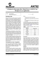
Tuan Giao area. The aeromagnetic data used in

this area is the aeromagnetic anomaly map on a
scale of 1:1,000,000 that was established and
published in 2005 by the General Department
of Geology and Minerals, bounded by longitude (103°E-104°E) and latitude (21°N368

22.3°N) according to geographic coordinate
system (Figure 9). Le Huy Minh et al. (2001)
used the method of horizontal gradient vector
field (HG) in combination with the reduction to
the pole to interpret this data with the aim of
determining magnetic boundaries of this area.
The values of magnetic anomalies in the area
vary from -350nT to 50nT, which are mainly
concentrated in the northeast of the area and
distributed in the northwest-southeast direction.
According to the geological data, this area has
the complex geological structure and strongest
seismic activity in the territory of Vietnam. In
the area, the major faults are the Dien Bien Lai Chau fault in the sub-longitudinal direction; the Son La fault, the Da River fault, the


Nguyen Thi Thu Hang, et al./Vietnam Journal of Earth Sciences 39 (2017)

Ma River fault, and other northwest-southeast
faults which are separated by the northeast-

southwest small faults (Cao Dinh Trieu, Pham
Huy Long, 2002).

nT

Figure 9. Aeromagnetic anomaly map ΔTa in Tuan Giao area;
Scale 1:1,000,000 (General Department of Geology and Minerals, 2005)

The study area also consists of many geological complexes (Geological and Mineral
Resources Map of Vietnam 1:200,000, the
sheets Mong Kha-Son La, Phong Sa Ly-Dien
Bien Phu, Kim Binh-Lao Cai, 2005) such as
Ma River complex, Phun Sa Phin complex,

Ngoi Thia volcanic complex, Tu Le volcanic
complex, Pu Sam Cap complex, etc. The
lithologic composition of these complexes is
very diverse. The Muong Hum complex consists of many types of high potassium calcalkaline rocks (monazite series) or subalkaline
369


Vietnam Journal of Earth Sciences, 39(4), 360-375 

granitic rocks. The Phun Sa Phin complex
consists of shallow and sub-volcanic intrusive
bodies of comagmatic granite and syenite together with rhyolitic-trachytic extrusive formations. The rocks in the Pu Sam Cap complex are mainly categorized into the alkaline
series; a few are categorized into the monazite
series. The rocks in these complexes are highly magnetic.
The determination of the structure of magnetic boundaries is carried out by calculating
the derivatives in different directions, then
computing the maximum values of new DG
function (|DGmax|). The positions of the maxima (|DGmax|) of total magnetic anomalies ∆Ta
is determined by the algorithm of Blakely &
Simpson presented above. In the figures

showing the calculation results, the positions
of (|DGmax|) are represented by black dots and
superimposed on the geological map of Tuan
Giao area (Geological and Mineral Resources
Map of Vietnam 1:200,000, the sheets Mong
Kha - Son La, Phong Sa Ly - Dien Bien Phu,
Kim Binh - Lao Cai, 2005).

3.3. With the gradient directions being the
longitudinal and northwest-southeast directions
The calculation results are represented in
Figure 10a, b, respectively. The results show
that with these gradient directions, the maxima of |DG| function (|DG|max) are concentrated
in small clusters and distributed sparsely, unsystematically. Very few clusters are located
along the faults, but they only extend to the
small, short and discontinuous segments. The
majority of clusters across the faults. Especially in the northwest and southwest of the
study area, there are no dots representing the
positions of |DG|max, although in this area
there are the Dien Bien - Lai Chau and Ma
River faults whose positions are also related
to magnetic boundaries (Le Huy Minh et al.,
2001). It shows that in case of using the new
DG function to determine boundaries of magnetic anomaly sources in Tuan Giao area, both
longitudinal and northwest-southeast gradient
directions are not appropriate to the geological
structure of Tuan Giao area.

Figure 10. Determination |DG|max of total magnetic anomalies ΔTa in Tuan Giao area at z = 0 km with the gradient
directions being the longtitudinal and northwest-southeast directions : a) Longtitudinal direction;

Faults;
Geological complexes)
b) Northwest Southeast direction ( Positions of |DG|max;

370


Nguyen Thi Thu Hang, et al./Vietnam Journal of Earth Sciences 39 (2017)

3.4. With the gradient direction being the
northeast-southwest
With this gradient direction, we have determined the positions of |DG|max of the total
magnetic anomalies ∆Ta at z = 0 and at different levels of upward continuation in order to
examine the relationship between the magnetic boundaries according to the depth of investigation.
At z = 0: The obtained result is represented
in Figure 11. The result shows that this is the
optimum gradient direction. Indeed, with this
gradient direction, in the figure showing its
result, the dots representing are distributed in
bands and clearly follow the northwestsoutheast direction. According to the geological data, the Dien Bien - Lai Chau fault in the
sub-longitudinal direction is located in the
northwest of the study area; according to the
result of calculating |DG|max, the positions of
|DG|max in this area are concentrated and
spread from north to south. In the south of this
fault, the position of |DG|max band is 5 km - 10
km far from the fault. In comparison with the
geological map and geological features of this
area, it can be seen that |DG|max occurs more
commonly because iron ores or blocks in this

area have the stronger magnetism than those
in the adjacent areas. In the center of the study
area, |DG|max occurs with high frequency and
is located along the Da River fault and the
majority of Son La fault in the northwestsoutheast direction. The Than Uyen fault is
located in the northeast of the study area; the
positions of |DG|max are mainly concentrated in
the east of this fault, in which there are granitic blocks, tuffaceous sandstone, rhyolite, felsite of the Ngoi Thia, Tu Le and Phun Sa Phin
volcanic complexes. The Ma River fault is located in the southwest and south of the study
area; the positions of |DG|max are concentrated
in the south of this fault, in which there is the
Ma River formation with highly magnetic
block. It is obvious that except for the magnetic boundary in the northwest following the

north-south direction, in general the magnetic
boundaries in the area determined by |DG|max
follow the northwest-southeast direction,
which is consistent with the main direction of
geological faults in the area. Compared to the
map of geological faults determined by the
research results of previous authors (Geological and Mineral Resources Map of Vietnam
1:200,000, the sheets Mong Kha - Son La,
Phong Sa Ly - Dien Bien Phu, Kim Binh - Lao
Cai, 2005), some magnetic boundaries determined by |DG|max almost coincide with the positions of major faults in the area: Dien Bien Lai Chau fault in the sub-longitudinal direction, Son La fault extending from the VietnamChina border below Phong Tho through Than
Uyen, Son La fault, Ma River fault, Than Uyen
fault. However, some positions of the faults do
not coincide completely with the positions of
|DG|max. This can be explained as follows. The
dot positions (the positions of |DG|max) reflect
the boundaries of blocks which can be observed on the surface, but they can also reflect

the deep boundaries which are not observed on
the fault map.
To eliminate the effect of shallow blocks
near the surface as well as to find magnetic
boundaries located at different depths, the calculation of |DG|max has been carried out at the
upward continuation to 2.5 km and 7.5 km.
The calculation results are represented in Figure 12, in which:
At the upward continuation to 2.5 km (Figure 12a): The calculation results show that
at this level of upward continuation, the
|DG|maxdistribution map most clearly shows the
magnetic boundaries which are located deeper
in the area. The separate, discrete maximum
points and the small, short |DG|max bands reflect
the small, shallow structures near the surface
that have disappeared. The maximum points
are clearly distributed in bands. Some structures such as the above-mentioned major extrusive masses and Son La fault, Da River fault,
Ma River fault are still obviously represented.
371


Vietnam Journal of Earth Sciences, 39(4), 360-375 

Especially, in the southwest of the study area
between longitude 103°E - 103.3°E and latitude 21°N - 21.3°N where the anomalies ΔTa
are stable and the contour lines are sparse, the
|DG| function has small value and the dots
representing the positions of |DG|max appear
infrequently. This can be because the geological complexes in this area begin from Nam Su
Lip through Na Khoang to Phu Sen Tung,
with Suoi Bang formation, Tay Trang formation and Nam Su Lip formation, which

consist mainly of sandstone, conglomerate,

schist with weak magnetization.
At the upward continuation to 7.5km (Figure 12b): At this level of upward continuation,
the density of the dots representing the positions of |DG|max significantly reduces, but they
are still distributed in bands and extend in the
northwest-southeast direction. At this level,
the maxima |DG|max only reflect the positions
of magnetic boundaries which are located
deeper and related to the major faults such as
Da River fault, Than Uyen fault, Son La fault,
Ma River fault.

Figure 11. Determination |DG|max of total magnetic anomalies ΔTa in Tuan Giao area at z = 0 km with the gradient
direction being the northeast-southwest ( Positions of |DG|max;
Faults;
Geological complexes)

372


Nguyen Thi Thu Hang, et al./Vietnam Journal of Earth Sciences 39 (2017)

Figure 12. Determination |DG|max of total magnetic anomalies ΔTa in Tuan Giao area with the gradient direction
Faults;
being the northeast-southwest: a) at z = 2,5 km; b) at z = 7,5 km ( Positions of |DG|max;
Geological complexes)

4. Discussions
From the calculation results based on numerical models as well as actual observation

data, in comparisons with the method of horizontal gradient vector field (HG) applied in
the same study area, it is possible to make the
following remarks on the applicability of the
method of the directional gradient (DG):
With the method of using the maximum
values of HG function, when the magnetized
object extends in one direction and has a narrow width, if the anomalies are not reduced to
the pole, the boundary of the object will not
be sufficiently determined, the two boundaries
in the extending direction of the object seem
to be reduced to a straight line coinciding with
the extending axis of the object (Figure 4a). It
is only fully determined in case the anomalies
are reduced to the pole before calculating HG
(Figure 4b). Meanwhile, according to the
maximum values of |DG| function (|DG|max),

the determination of the boundary of the
source is completely independent of the magnetization inclination of the source; even in
case the anomalies are not reduced to the pole,
the two boundaries in the extending direction
of the source are sharply and clearly represented (Figure 4c, d).
When many sources are located in the
study area or they cross each other, the method of using the maximum values of DG function still completely and sharply defines the
boundaries of all objects, even if the field is
not reduced to the pole. It indicates that this
method is not affected by interference. The
calculation results also show that this method
is slightly affected by noise.
Based on the calculation with actual magnetic anomaly data in Tuan Giao area, we

have found that in case of applying the directional gradient (DG) and selecting the appropriate gradient direction, although the reduc373


Vietnam Journal of Earth Sciences, 39(4), 360-375 

tion to the pole is not carried out, the calculation results show the concordance between the
structural direction as well as positions of
magnetic boundaries in the area determined
by |DG|max and the results of magnetic data
analysis when using maximum horizontal
gradient vector field (HG) of magnetic
anomalies in Tuan Giao area after reduction to
the pole and upward continuation to 2.5 km
(Le Huy Minh, Luu Viet Hung, Cao Dinh
Trieu, 2001). Moreover, according to this
method (DG), the positions of magnetic
boundaries extend continuously and are represented more clearly than in the HG method.
This further confirms the reliability of directional gradient of total magnetic anomalies in
the analysis of actual data.
5. Conclusions
By studying and applying the directional
gradient of magnetic anomaly field to determine the boundaries of magnetized objects
based on numerical models as well as actual
magnetic anomaly data in Tuan Giao area, it
is possible to make the following remarks:
In case the magnetic anomaly sources are
narrow in width and their structure extends in
one direction, the boundaries of the sources
can be completely determined by the method
of the directional gradient. With this method,

according to the maximum values of DG
function (|DG|max), the determination of the
boundaries of the sources does not depend on
the magnetization inclination of the sources.
In cases of vertical magnetization and inclined
magnetization, the boundaries of the sources
are sharply and clearly represented. Meanwhile, when using the method of horizontal
gradient vector field, the boundaries of the
sources are only represented completely in
combination with the reduction to the pole.
However, this intermediate step will result in
significant errors in the processing, especially
in case the study area is located in a lowlatitude region.
374

In addition, with this method, the interference which occurs in complex conditions with
insignificant differentiation is also eliminated.
The positions and shapes of magnetized objects are still precisely determined, even if
they cross each other or the noise appears.
The experimental results on the models show
that even when the random noise mixed in
anomalies has the maximum value of ±14nT
(±1% ΔTmax), the boundaries of the sources
are still determined with high sharpness.
The application of directional gradient in
the analysis of aeromagnetic anomaly field in
Tuan Giao area shows that the magnetic
boundaries in the area basically follow the
northwest-southeast direction, which is consistent with the main direction of geological
faults in the area. The positions of some magnetic boundaries almost coincide with those of

major faults in the area (Da River fault, Son
La fault, Than Uyen fault). This indicates a
connection between these geological faults
and the magnetic susceptibility of associated
formations.
The calculation results based on the models as well as the actual data demonstrate the
applicability of directional gradient in interpreting magnetic anomaly data in Vietnam. It
is particularly effective in interpreting magnetic anomaly data in the areas where the
magnetic boundaries extend in one direction.
References
Bhaskara Rao D. and N. Ramesh Babu, 1993. A fortran
77 computer program for tree dimensional inversion
of magnetic anomalies resulting from multiple prismatic bodies, Computer & Geosciences, 19(8),
781-801.
Beiki M., David A. Clark, James R. Austin, and Clive A.
Foss, 2012. Estimating source location using normalized magnetic source strength calculated from
magnetic gradient tensor data. Geophysics, 77(6),
J23-J37.
Blakely R.J., and R. W. Simpson, 1986. Approximating
edges of source bodies from magnetic or gravity
anomalies: Geophysics, 51, 1494 -1498.
Blakely R.J., 1995. Potential theory in gravity and magnetic applications, Cambridge University Press.


Nguyen Thi Thu Hang, et al./Vietnam Journal of Earth Sciences 39 (2017)
Cao Dinh Trieu, Pham Huy Long, 2002. Tectonic fault
in Vietnam. Publisher of Science and Engineering.
Debeglia N. and J. Corpel, 1997. Automatic 3-D interpretation of potential field data using analytic signal
derivatives. Geophysics, 62, 87-96.
Geological and Mineral resources map on 1:200,000.

Seriesof Tay Bac, sheets of Muong Kha - Son La (F48-XXV-F-48-XXVI), Phong Sa Ly - Dien Bien
Phu (F-48-XIX-F-48-XX), Kim Binh - Lao Cai (F48-VIII-F-48-XIV), 2005. Published and copyringt
by Department of Geology and Minerals of
Vietnam, Hanoi.
Le Huy Minh, Luu Viet Hung, Cao Dinh Trieu, 2001.
Some modern methods of the interpretation
aeromagnetic data applied for Tuan Giao region.
Vietnam Journal of Earth Sciences, 22(3), 207-216.  
Le Huy Minh, Luu Viet Hung, Cao Dinh Trieu, 2002.
Using the maximum horizontal gradient vector to interpret magnetic and gravity data in Vietnam.
Vietnam Journal of Earth Sciences, 24(1), 67-80.
Nabighian M.N., 1972. The analytic signal of twodimensional magnetic bodies with polygonal crosssection: Its properties and use of automated anomaly
interpretation: Geophysics, 37, 507-517.

Nabighian M.N., 1974. Additional comments on the
analytic signal of two-dimensionalmagnetic bodies
with polygonal cross-section. Geophysics, 39, 85-92.
Roest W. R., J. Verhoef and M. Pilkington, 1992. Magnetic interpretation using the 3-D analytic signal:
Geophysics, 57, 116-125.
Vo Thanh Son, Le Huy Minh, Luu Viet Hung, 2005.
Three-dimensional analytic signal method and its
application in interpretation of aeromagnetic
anomaly maps in the Tuan Giao region. Proceedings
of the 4th geophysical scientific and technical
conference of Vietnam, Publisher of Science and
Engineering 2005.
Vo Thanh Son, Le Huy Minh, Luu Viet Hung, 2005.
Determining the horizontal position and depth of the
density discontinuties in Red River Delta by using
the vertical derivative and Euler deconvolution for

the gravity anomaly data, Journal of Geology, Series
A, 287(3-4), 39-52.
Vo Thanh Son, et al., 2007. Determining the location
and depth of contrast magnetic boundaries by using
3D analytics signal method and higher derivatives.
Proceeding of the 5th geophysical scientific and
technical conference of Vietnam.

375