TEC variations and ionospheric disturbances during the magnetic storm in march 2015 observed from continuous GPS data in the southeast asia region VJES 38

Vietnam Journal of Earth Sciences Vol 38 (3) 287-305
Vietnam Academy of Science and Technology

Vietnam Journal of Earth Sciences
(VAST)

/>
TEC variations and ionospheric disturbances during the
magnetic storm in March 2015 observed from continuous
GPS data in the Southeast Asia region
Le Huy Minh*1, Tran Thi Lan1, R. Fleury2, Le Truong Thanh1, Nguyen Chien Thang1,
Nguyen Ha Thanh1
1

Institute of Geophysics, Vietnam Academy of Sciences and Technology
Lab-STICC, UMR 6285 Mines-Télécom, Télécom Brest, France

2

Received 7 April 2016. Accepted 15 August 2016
ABSTRACT
The paper presents a method for computing the ionospheric total electron content (TEC) using the combination of
the phase and code measurements at the frequencies f1 and f2 of the global positioning system, and applies it to study
the TEC variations and disturbances during the magnetic storm in March 2015 using GPS continuous data in the
Southeast Asia region. The computation results show that the TEC values calculated by using the combination of
phase and code measurements are less dispersed than the ones by using only the pseudo ranges. The magnetic storm
whose the main phase was on the 17th March 2015, with the minimum value of the SYM/H index of -223 nT is the
biggest during the 24th solar cycle. In the main phase, the crests of the equatorial ionization anomaly (EIA) expanded
poleward with large increases of TEC amplitudes, that provides evidence of the penetration of the magnetospheric
eastward electric field into the ionosphere and of the enhancement of the plasma fountain effect associated with the
upward plasma drifts. In the first day of the recovery phase, due to the effect of the ionospheric disturbance dynamo,

the amplitude of northern crest decreased an amount of about 25% with respect to an undisturbed day, and this crest
moved equatorward a distance of about 11o, meanwhile the southern crest disappeared completely. In the main phase
the ionospheric disturbances (scintillations) developed weakly, meanwhile in the first day of the recovery phase, they
were inhibited nearly completely. During the storm time, in some days with low magnetic activity (Ap<~50 nT), the
ionospheric disturbances in the local night-time were quite strong. The strong disturbance regions with ROTI > 0.5
concentrated near the crests of the EIA. The latitudinal-temporal TEC disturbance maps in these nights have been
established. The morphology of these maps shows that the TEC disturbances are due to the medium-scale travelling
ionospheric disturbances (MSTID) generated by acoustic-gravity waves in the northern crest region of the EIA after
sunset moving equatorward with the velocity of about 210 m/s.
Keywords: Total electron content (TEC), equatorial ionization anomaly (EIA), medium-scale traveling
ionospheric disturbance (MSTID).
©2016 Vietnam Academy of Science and Technology

1. Introduction1
In the middle of March 2015, the biggest
magnetic storm during the 24th solar cycle
*

occurred with the value of the SYM/H index
of -223 nT. The main phase of the storm was
on 17 March, so it was called the Saint
Patrick’s Day storm. The storm is caused by
the outbreak of chromosphere-type X, the

Corresponding author, Email:

287


L. H. Minh, et al./Vietnam Journal of Earth Sciences 38 (2016)

extremely strong one, which is derived from a
black line in the active zone named AR12297,
observed on 11 March. According to the
scientists of the Space Weather Prediction
Center (SWPC), the storm can lead to
the disruption of high-frequency radio
transmission for hours in several large areas.
It is known that during the time of magnetic
storm, the ionospheric electric field
disturbances observed in the medium and low
latitude regions have different timescales,
strongly influence the distribution of
ionospheric plasma, originate from the direct
penetration of the magnetospheric electric
field into the ionosphere (Nishida, 1968;
Vasiliunas, 1970, 1972; Jaggi & Wolf, 1973;
Fejer et al., 1979, 1990; Gonzales et al., 1979;
Kelley et al., 1979, Spiro et al., 1988;
Peymirat & Fontaine, 1994; Fejer &
Scherliess, 1995; Foster & Rich, 1997;
Kikuchi et al, 2000; Kelley et al., 2003; Fejer
& Emmert, 2003) and the effects of
ionospheric disturbance dynamo last longer
(Blanc & Richmond, 1980; Spiro et al., 1988;
Sastri, 1988; Fejer & Scherliess, 1995; FullerRowell et al., 2002; Richmond et al., 2003).
In the storm time, the basic elements of
ionospheric effects in low latitude regions are
generated by the morphological change of the
equatorial

ionization
anomaly,
EIA,
(Appleton, 1946). During the storm, the
ionospheric disturbances can appear in the
night-time due to the traveling ionospheric
disturbances (TIDs) that are the waveform
disturbances
of
ionospheric
plasma
(Afraimovich et al., 2013; Hines, 1960). There
are two types of TID having almost periodic
oscillations (Georges, 1968): large-scale TID
(LSTID) characterized by high velocity (>
300 m/s) and long cycle (> 1h) and mediumscale TID (MSTID) characterized by lower
speed (50-300 m/s) and shorter cycle (10 min
to 1h). LSTIDs appear as a chain of shortwave
with the small number of cycles, meanwhile,
MSTIDs can have several cycles (Francis,
1974). In addition to the mentioned TIDs,
there are MSTIDs having no cycle that appear
as the oscillations with different cycles of the
electron density. MSTIDs are present in the F
288

region of the ionosphere, whereas LSTIDs are
much scarcer, only appear in case of the big
magnetic storms. LSTIDs originate from the
auroral region (Georges, 1968; Davis, 1971)

while the observations of MSTIDs suggest
that their source mechanisms are in the lower
latitude regions (Munro, 1958; Davies &
Jones, 1971). Many studies on TID based on
observation of the ionospheric total electron
content (TEC) from the dense network of GPS
stations in Japan (Saito et al., 1998; Shiokawa
et al., 2002; Afraimovich et al., 2009), in
North America (Tsugawa et al., 2007), in
Europe (Borries et al., 2009), and from the
chain of GPS stations in the region of AfricaEurope Shimeis et al. (2015) have also
observed the signs of TID in the medium and
low latitude regions. This paper presents the
observation results of TEC variations and
ionospheric disturbances from GPS data in
Vietnam and the Southeast Asia region during
the magnetic storm occurring from 15 March
to 28 March 2015.
2. Data and calculation method
Data used in this paper are from the
continuous GPS stations in Vietnam and the
Southeast Asia region, whose names,
magnetic coordinates and latitudes are listed
in Table 1 and presented in Figure 1. From
XMIS to PHUT the latitudes change from 19.58o to 14.89o, so that we can obtain
information about the equatorial ionization
anomaly in the Southeast Asia region (Le Huy
et al., 2014). Among these 8 stations, PHUT
and HUE2 stations with GSV4004 receiver
can provide the S4 indices, the standard

deviation of the code/carrier phase (ccd), the
specific parameters of the amplitude
scintillation of GPS signals when traveling
through the ionosphere.
To calculate TEC, a method of using the
pseudo range measurements is presented in
(Le Huy et al., 2014; Le Huy Minh et al.,
2006), in this paper we introduce the method
of using the combination of the phase and
pseudo range measurements.


Vietnam Journal of Earth Sciences Vol 38 (3) 287-305

Figure 1. Location of GPS receivers and traces of the visible satellites at 400km altitudes on the 15 March 2015

289


L. H. Minh, et al./Vietnam Journal of Earth Sciences 38 (2016)
Table 1. GPS stations in Vietnam and Southeast Asian region
Geographic coordinate
No
Station
Receiver
Latitude
Longitude
1
PHUT
GSV4004

21.02938
105.95872
2
VINH
CORS5700
18.64999
105.69659
3
HUES
GSV4004
16.45883
107.59346
4
TNGO
CORS5700
15.44722
108.20385
5
CUSV
NETRS
13.73591
100.53392
6
DLAT
JAVAD
11.94526
108.48173
7
NTUS
LEICA

1.34580
103.67996
8
BAKO
LEICA
-6.49106
106.84891
9
XMIS
NETR9
-10.44997
105.68849

In the dual frequency GPS measurements,
the pseudo range measurement p kji and the
phase measurement Likj at the GPS

Magnetic Latitude
(2015)
14.89
12.32
9.58
8.92
6.86
5.16
-6.62
-15.10
-19.58

frequencies f1 and f2 are measurable, so they

can be written (Liu et al., 1996; Carrano &
Groves, 2009):

i
i
i
i
p
p
p1i j  s0i j  dion
1 j  dtropj  c(   j )  bp1  bp1 j  m1  1

i
i
i
i
p
p
p2i j  s0i j  dion
2 j  dtropj  c(   j )  bp 2  bp 2 j  m2   2

i
i
i
i
i


L1i j  s0i j  d ion
1 j  d tropj  c(   j )  b 1  1 N1 j  m1   1

(1a)
(1b)
(1c)

i
i
i
i
i


Li2 j  s0i j  dion
2 j  dtropj  c(   j )  b 2  2 N 2 j  m2   2 (1d)

where i and j indices are the satellite i and the
receiver j respectively; s0 is the real distance
between the receiver and the satellite, dion and
dtrop are the ionospheric delay and the
tropospheric delay, c is the speed of light in
vacuum,  is the satellite clock error or the
receiver clock error, b is the device delay of
the satellite or of the receiver, N is the
multivalued integer,  is the transmission
wavelength, m is the multipath effect in the
pseudo range measurements or in the phase
measurements,  is the interference in the
corresponding
measurements
at

the
frequencies f1 and f2.
According to the Appleton formula
(Budden, 1985), the ionospheric delay
conforming to slant total electron content

(STEC) between the Rx receiver and the Tx
satellite can be written:
40,3
40,3
1 
d ion  s   s0     1dl  2  N (l )dl  2 STEC (2)
n
f
f

Tx 
Tx
Rx

Rx

where s’ is the apparent distance between the
receiver and the satellite, N (l) is the electron
density along the satellite-receiver line in
el/m3, n is the refractive index, and f is the
frequency of radio waves in Hz.
The ionosphere acts as the scattering
medium for GPS signals, but the troposphere
is the non-scattering medium, so the

tropospheric delay can be eliminated by using
the subtraction (1b)-(1a) and (1c)-(1d). Using
the subtraction (1b)-(1a) and ignoring the
multipath effect and the interference, we have:

i
i
i
i
i
i
i
p2i j  p1i j  d ion
2 j  d ion1 j  (b p 2  b p1 )  b p 2 j  b p1 j   d ion 2 j  d ion1 j  b p  b pj

290

(3)


Vietnam Journal of Earth Sciences Vol 38 (3) 287-305

By the combination of the formulas (2) and
(3) we have:
STEC 



1
f12 f 22

p2i j  p1i j  (bip  bpj )
40,3 f12  f 22



(4)

Using the subtraction (1c)-(1d) and
ignoring the multipath effect and the
interference, we have:





i
i
i
i
i
i
L1i j  Li2 j  dion
1 j  d ion 2 j  (b1  b2 )  b1j  b2j   1 N1 j  2 N 2 j 



i
i
i
i

i
 dion
1 j  d ion 2 j  b  bj  1 N1 j  2 N 2 j



Combining (2) with (5) we have:
f12 f 22
1
L1i j  Li2 j   bi  bj   1 N1i j  2 N 2i j 
STEC 
40,3 f12  f 22
In the formulas (4) and (6) STEC is
calculated in TECU, 1TECU  1016 el / cm 3 .
The vertical total electron content, VTEC or
written as TEC, observed at the breakpoint of
the ionosphere is determined from singlelayer model (Klobuchar, 1986):


 R cos 
TEC  STEC. cosarcsin
 (7)
 R  h 


where  is the satellite elevation angle in
degree (o), R = 6371.2 km is the average
radius of the Earth, h is the height of
ionospheric single layer, often considered as
400 km (Zhao et al., 2009).

So, to work out the value of STEC from
the formula (4) we need to calculate the
device delays bp  bip  bpj (the constant for
each pair of satellite-receiver), from the
formula (6) we need to calculate the device
b  bi  bj
and
the
nondelays
determination of initial phase 1 N1i j  2 N 2i j

that are also the constants.
In

STEC p 

1  f f

40,3  f  f 22
the

 i
 p 2 j  p1i j  is a


formula

2
1
2

1

2
2

(4),

quantity that is clearly determined, however
due to the influence of interference and
multipath effect, its values are usually
dispersed; and in the formula (6), the quantity

1  f12 f 22

STEC 
40,3  f12  f 22

 i
L1 j  Li2 j 


is

(5)

(6)

precisely determined but suffers the jumps
due to the cycle slip (Carrano & Groves,
2009). We use the quantity STECp to

eliminate the jumps in the STEC as follows.
Within each continuous distance of the
satellite tracks, STECp is approximated by the
fourth-degree polynomial. The quantity
STEC is compared with STECp, which is
smoothed by polynomial approximation, to
evaluate the magnitude of the jumps in STEC
on the same satellite track. VTEC in case of
regulating the jumps is calculated and
compared with the value of VTEC from the
global TEC model (CODG model) at the
corresponding time in order to determine the
total delay of device delay and the nondetermination of initial phase that is similar to
the estimation of device delay in calculating
the absolute TEC by using the pseudorange
measurements. The value of total delay for
each pair of satellite-receiver in the
observation day is the average value of total
delay at each observation time. To reduce
multipath effect in the low satellite elevation
angles, the values of TEC used to compare
with TEC from the global model are often
chosen in accordance with the satellite
elevation angle α ≥ 30o.
To study the ionospheric scintillation from
data of the receiver GSV4004, we use the
amplitude scintillation index S4 that is
calculated according to the formula (Van
Dierendonck et al., 1993):

S 4  S 42tot  S 44cor

(8)
291


L. H. Minh, et al./Vietnam Journal of Earth Sciences 38 (2016)

where S4tot is the total S4 and S4cor is the
corrected S4 due to the interference effect.
Both of these quantities are obtained directly
from the output signal of the receiver
GSV4004. S4 obtained in such way contains
the multipath effect, especially in low satellite
elevation angle, therefore the scientists often
rely on the parameter ccd, which characterizes
the influence of multipath effect, to establish a
filter limit for each station (Tran Thi Lan et
al., 2011; Abadi et al., 2014; Tran Thi Lan et
al., 2015). The method is based on selecting
days of quiet ionosphere in each year at each
station, graphing the relationship between the
parameter ccd and the index S4, finding a line
to separate the scintillation due to multipath
effect from the one due to the ionosphere,
then the S4 indices over this line are supposed
to be caused by multipath effect, and the ones
under this line are supposed to be caused by
ionospheric effect. Applying such filter limit
on days of any data at each station, we obtain

the index S4 caused by the ionospheric
scintillation. The index S4 obtained in such
way is S4 for the different satellite elevation
angles, to get the vertical S4, we apply the
formula (Spogli et al., 2009):

S4 (  90o )  S4 ( ) sinb ( )

(9)
where α is the satellite elevation angle, b is
chosen to be 0.9.
Another index indicating the level of
ionospheric disturbance - ROT, which is the
rate of change of TEC with respect to time
calculated from the L1 and L2 phase
measurements, is used (Pi et al., 1997):

ROT 

VTECuk  VTECuk1
tu  tu 1

(10)

where k is the visible satellite, u is the time of
observation and ROT is calculated in
TECU/minute. The measurements of ROT
point out the small-scale variations on the
background of a larger-scale trend. The rate of
TEC index, ROTI, is defined as the standard

deviation of ROT at 5-minute interval:
ROTI 

292

ROT 2  ROT

2

(11)

Ordinarily, ROTI ≥ 0.5 reveals the presence of
ionospheric anomalies on the scale of a few
kilometers or more (Ma & Maruyama, 2006).
3. Calculation results and discussion
3.1. Magnetic parameters during storm time
Figure 2 represents the component X of the
solar wind Vx, the component Z of
the interplanetary magnetic fields Bz, the
symmetric disturbance field in H index
SYM/H and the auroral electrojet index AE
between 15 March and 28 March 2015, in
which Vx and Bz are moving-averaged in the
period of an hour. It is necessary to note that
the time in each day of the dataset is based on
the universal time (UT), the local time LT
equals the UT plus 7, in the figure there are
two vertical lines corresponding to the start
times of the main phase and the recovery
phase of the storm examined. At 18:00 UT on

15 March Vx began to increase from 295 km/s
and reached a maximum of about 690 km/s at
the end of 18 March. Vx ranged between 550
km/s and 690 km/s from 18 to 25 March; in
three following continuous days of 26-28
March Vx decreased from 550 km/s to 400
km/s. In the period of 15-28 March, except for
March 17, Bz varied from -7 nT to ~11 nT. On
17 March Bz unexpectedly changed from 8
nT at 3:17 UT to 21.6 nT at 4:34 UT; then Bz
suddenly reduced from positive value to
negative value, which was essentially the
movement of Bz from the northward direction
to the southward direction; and in most of
time between 4:43 UT and 23:12 UT Bz was
toward the South; but in 2 periods of 6:09 UT
- 6:33 UT and 8:49 UT - 11:27 UT, Bz was
toward the North. The index Dst demonstrates
that the main phase occurred on 17 March
from 5:00 UT to 23:00 UT; the minimum
value of SYM/H index of -223 nT indicates
that it was the big storm. The recovery phase
started after the main phase from ~ 23:00 UT;
the SYM/H index began to increase in
accordance with the movement of Bz from the


Vietnam Journal of Earth Sciences Vol 38 (3) 287-305

South to the North. The variations of SYM/H

index show that until the end of 28 March the
value of SYM/H index almost came back to
that on 15 March, thus the recovery phase of
this storm completed at the end of 28 March.
In the main phase of the storm, the AE index
rose to a peak of 1570 nT; between 18 March

and 28 March, the maximum of AE index was
from 1130 nT on 19 March to 408 nT on 27
March. In the main phase of the storm, the
magnetic activity index Ap reached the
maximum of 179 nT, 80 nT, 94 nT on 17, 18
and 22 March respectively; and on other days,
the Ap index was smaller than 50 nT.

-300

Vx (km/s)

-400
-500
-600
-700
15

16

17

18

19

20

21

22

23

24

25

26

27

28

29

15

16

17

18

19

20

21

22

23

24

25

26

27

28

29

15

16

17

18

19

20

21

22

23

24

25

26

27

28

29

15

16

17

18

19

20

21

22

23

24

25

26

27

28

29

15

16

17

18

19

20

21
22
23
24
Day, March 2015

25

26

27

28

29

30
20

Bz (nT)

10
0
-10
-20

-30

SYM/H (nT)

50
0
-50
-100
-150
-200

1600

AE (nT)

1200
800
400

Kp

0
9
8
7
6
5
4
3
2

1
0

Figure 2. From top to bottom, X-component of solar wind speed (Vx), z-component of the IMF (Bz), symmetric
disturbance field in H index (SYM/H), auroral magnetic index (AE) and planetary Kp are displayed. The main phase
of the storm is limited in two vertical solid lines

293


Vietnam Journal of Earth Sciences Vol 38 (3) 287-305

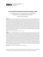
3.2. TEC variations
To compare the calculation result of TEC
from the pseudo range measurements and that
from the combination of the phase and pseudo
range measurements as mentioned above,
Figure 3 presents the computation results of
TEC by both methods for data at Phu Thuy
GPS station on 1 January 2012. It can be seen
that the shapes of the TEC curves calculated
from both types of data are identical. However
it is obvious that on each satellite line the

values of TEC obtained from the method
presented here are less dispersed. It indicates
that the values of TEC computed by using the
combination of phase and pseudo range
measurements are more reliable than those by
using the pseudo range measurements, as

some other authors in the world have noticed
(Liu et al., 1996, Carrano & Groves, 2009).
The calculation method of TEC presented
above is applied to the dataset of GPS stations
in the Southeast Asia region in the period
from 15 to 28 March 2015.

Figure 3. Total electron content on the 15 March 2015 computed a) by using pseudorange measurements, and b) by
using the combination of carrier phase and pseudorange measurements

Figure 4 presents the temporal-latitudinal
maps of TEC in the Southeast Asia region
between 15 and 28 March 2015. In Figure 4
the location of the magnetic equator is
indicated by the line in the latitude of 7-8oN.
294

The maps in Figure 4 clearly shows the
structure of the equatorial ionization anomaly
in the Southeast Asia region, including a crest
in the northern hemisphere and another in
the southern hemisphere that is almost


Vietnam Journal of Earth Sciences Vol 38 (3) 287-305

symmetrical to each other over the magnetic
equator. The morphology of anomaly changed
continuously day by day during the storm.
Figure 5 presents the amplitude, appearance

time and latitude of the corresponding
anomaly crest in that period. The amplitudes
of anomaly on 16 and 17 March rose
markedly, the crest expanded poleward and
the appearance time was earlier than that on
15 March. On 18 March, the beginning day of
the recovery phase, the anomaly degenerated,
only the northern crest existed with the
amplitude decreasing remarkably (about
25%), it moved equatorward a distance of 11o
compared to that on 17 March and its
appearance time was a few hours earlier than
that on 19 and 17 March, meanwhile the
southern crest completely disappeared. The
complete disappearance of the southern crest
of the equatorial ionization anomaly was also
observed by Lin et al. (2005) in the big
magnetic storm within September-October
2003. In the first phase of the magnetic storm,
the vertical component of the interplanetary
magnetic field Bz0, the interactions between
the solar wind and the southward

interplanetary magnetic field cause the
eastward electric field to penetrate directly
into the ionosphere (for example, Nishida,
1968; Kikuchi et al., 2000; Fejer & Emmert,
2003). This eastward electric field increases
the fountain effect as well as the amplitude
of anomaly crest and promotes the poleward

expansion of the anomaly crest. In the storm
when the high-energy particle flow of the
solar wind deeply penetrates into the
polar atmosphere and heats it, there is
the appearance of the meridian neutral
wind blowing equatorward. The complex
interactions between the neutral wind and
the Earth’s magnetic field cause the
phenomenon
called
the
ionospheric
disturbance dynamo (Blanc & Richmond,
1980) in which the electric field in the low
latitude region is in the westward direction,
in contrast to the eastward electric field in
normal condition. This westward parallel
electric field appears in the recovery phase,
causing the downward plasma drift, the
decrease in the fountain effect and the
degeneration of the structure of the
equatorial ionization anomaly.

Figure 4. Time and latitudinal TEC maps for the period between 15 and 28 March 2015. Contour interval: 5TECu.
SSC: sudden commencement of the storm, RP: the beginning of the recovery phase

295


L. H. Minh, et al./Vietnam Journal of Earth Sciences 38 (2016)

120
100
20

90
80
70
60
15 16 17 18 19 20 21 22 23 24 25 26 27 28
11
10

Time (UT)

c)
24

b)

9
8

Geographic latitude (degree)

TEC (TECu)

110

28

a)

16
12
8
4
0
-4

7
-8

6
5

-12
15 16 17 18 19 20 21 22 23 24 25 26 27 28
Day, March 2015

15 16 17 18 19 20 21 22 23 24 25 26 27 28
Day, March 2015
Figure 5. a) Maximum TEC, b) appearance time and c) latitude of the northern (black cycle) and southern (open
rectangular) EIA crests from 15 to 28 March 2015

3.3. Ionospheric disturbances
Figure 6 shows the variations of ROTI≥
0.5 at Hue station and ROTI≥0.575 at Phu
Thuy station (ROTI below this level appears
in almost all the observation times, and such
ROTI index does not reflect the disturbances

in the ionosphere), and the S4 indices selected
and calculated as presented above at Phu
Thuy and Hue stations from 15 to 28 March
2015. Figure 7 indicates ROTI ≥0.5 at TNGO,
CUSV, DLAT, NTUS, BAKO and XMIS
stations in that period. Figure 6 demonstrates
the definite correlation between the amplitude
scintillation index S4 and the index ROTI
calculated from the total electron content
obtained from the phase measurements,
although the numerical values of these indices
are different. These indices almost appear at
the night-time from 12:00 UT to 18:00 UT
(i.e. from 19:00 LT to 01:00 LT of the
following day). In the period studied, on 16,
19, 24-28 March the extremely strong
ionospheric disturbances were observed at
296

both stations, on 17, 18, 20-25 March very
few ionospheric disturbances were observed
at both stations, on 15 and 25 March the
ionospheric disturbances observed at Hue
stations were much more than those at PHUT
station. The distance between HUE and
PHUT is about 500 km, the ionospheric
anomalies at two stations have the same and
different characteristics that indicate the
spatial scales of the ionospheric anomalies are
not identical on the different days. We also

observe a similar condition in Figure 7. The
ROTI indices at five stations (TNGO, CUSV,
DLAT, NTUS and BAKO) on 16, 19, 24-28
March show that the ionospheric disturbances
observed at these stations were obvious. In
XMIS station, the furthest station from the
equator in the southern hemisphere, the
ionospheric disturbances observed were rather
plenty on 16 and 26 March as in other
stations, on other days the ionospheric
disturbances were also observed but
ROTI≥0.5 rarely appeared. In all eight
stations during the night of 18 March, the


Vietnam Journal of Earth Sciences Vol 38 (3) 287-305

ionospheric disturbances hardly appeared. As
mentioned above, on 18 March the
ionospheric disturbance dynamo developed,
the EIA degenerated, the southern crest of the
anomaly disappeared, the northern crest
moved equatorward a distance of about 11o
compared to that on 17 March; therefore,
when the ionospheric disturbance dynamo
developed, the westward electric field was
enhanced, causing the ionospheric F-layer to
move downward and the ionospheric
disturbances to be prevented. On 17 March,
the developing day of the main phase, due to

the direct penetration of the magnetospheric
eastward electric field into the ionosphere, the
equatorial ionization anomaly was enhanced;
the amplitude of the crest increased compared
to that on 16 March; the crest expanded
poleward; the appearance time of the
maximum was later; however, it can be seen
in Figure 6 and Figure 7 that the ionospheric
disturbances in the night of 17 March poorly
or hardly developed. On 16, 19, 24-28 March
the appearance of the values ROTI≥0.5 were
almost observed in all the stations, the
magnetic activity index Ap reached 48 nT on
19 March and was less than or equal to 22 nT
on other days, so on the appearance days of
the ionospheric disturbances; the magnetic
activity was relatively weak. To study the
spatial distribution of the ionospheric
disturbances, Figure 8 indicates the
distribution of the ROTI indices observed in
the night-time of 16 and 19 March, a day
before the main phase and a day in the
recovery phase of the storm, Figure 9 shows
the latitudinal distribution of the indices
ROTI≥0.5 on these two days. On 16 and 19
March the northern and southern crests were
in the latitudes of 22.4oN, 23.4oN and 8.0oS,
10.0oS respectively, the location of the
equator was in the latitude of about 7.8oN.
Accordingly, Figure 8 and Figure 9

demonstrate that the indices ROTI ≥0.5
mostly concentrated in the latitude of 16oN

and 6oS, the location of the maximum
disturbances (at night) concentrated closer to
the equator than the crest of the equatorial
ionization anomaly did (by day).
To examine the effects of TEC
disturbances, we determine the components of
TEC disturbances according to the formula:

TEC  TEC  TEC tb 2 h

where TECtb2h is the value of TEC in the
corresponding time that is moving-averaged
in the period of two hours, this process has
been used by many authors in order to analyze
the medium-scale and large-scale TIDs (Saito
et al., 1998; Borris et al., 2009). In some cases
when the disturbances have the shorter cycles
than we choose, the period of the moving
average is 30 minutes (Figure 10) or 1 hour.
The separation of the disturbance components
is executed for each satellite, then
the temporal-latitudinal maps of TEC
disturbances are established by the same
process as those of TEC. The results of
establishing TEC disturbance maps in the
night-time of 16, 19, 24-28 March 2015 are
presented in Figure 11.

The TEC disturbances maps are
established for the period from 12:00 UT to
24:00 UT (from 19:00 LT to 07:00 LT of the
next day) because the disturbances mainly
appear in this period (Figure 6 and Figure 7).
Although the amplitude of TEC disturbances
is small compared to that of TEC, but the
obtainment of the TEC disturbance maps
having the almost unified characteristics in
Figure 11 allows affirming that the process of
obtaining TEC disturbances as presented
above is logical. The TEC disturbance maps
in Figure 11 have the similar forms, two
positive disturbance regions are at two sides
of the magnetic equator, the negative
disturbances are in the magnetic equator and
adjacent regions, the negative disturbance
region near the magnetic equator in the south
is larger than that in the north. In the period
from 20:00 UT to 24:00 UT (03:00 LT-07:00
LT) the negative disturbances are mostly in
297


L. H. Minh, et al./Vietnam Journal of Earth Sciences 38 (2016)

ROTI (TECu/min)

the latitude region of 8oS-24oN. Figure 4
shows that on the TEC map the equatorial

ionization anomaly are nearly symmetrical
over the magnetic equator, meanwhile, on the
TEC disturbance map (Figure 11) the
symmetry of two disturbance regions at two
sides of the magnetic equator is less apparent.
In the north of the magnetic equator, the
positive disturbance regions stretching
continuously in the dashed line direction in
Figure 11 give us the picture of the
ionospheric disturbances moving equatorward
from the northern anomaly crest region. With
the scale of about 200-300 km as in Figure 11,
5
4

a)

3
2
1
0

1.0
0.8
S4

these disturbances can be considered
the medium-scale traveling ionospheric
disturbances (MSTID). Furthermore, Figure
10 shows that the TEC disturbance containing

several cycles with different wavelengths is
also a characteristic of MSTID. If the dashed
line direction in Figure 11 is considered to
indicate the movement direction of MSTID,
the movement velocity of the disturbances on
the examined days can be calculated at about
210 m/s toward the south. The apparent
asymmetry of the TEC disturbance regions in
Figure 11 suggests that maybe these MSTIDs
do not move across the magnetic equator.

a')

0.6
0.4

ROTI(TECu/min)

0.2
0.0
5
4

b)

3
2
1
0
1.0

b')

S4

0.8
0.6
0.4
0.2
15

16

17

18

19

20

21

22

23

24

25

26

27

28

Day, March 2015
Figure 6. ROTI and S4 indices a) and a’) at PHUT and b) and b’) at HUES from 15 to 28 March 2015

298

29


ROTI (TECu/min)

ROTI (TECu/min)

ROTI (TECu/min)

ROTI (TECu/min)

ROTI (TECu/min)

ROTI(TECu/min)

ROTI(TECu/min)

Vietnam Journal of Earth Sciences Vol 38 (3) 287-305

5
4
3
2
1
0
5
4
3
2
1
0
5
4
3
2
1
0
5
4
3
2
1
0
5
4
3
2
1
0

5
4
3
2
1
0
5
4
3
2
1
0

VINH

TNGO

CUSV

DLAT

NTUS

BAKO

XMIS

15

16

17

18

19

20

21

22

23

24

25

26

27

28

29

Day - March 2015
Figure 7. From top to bottle ROTI0.5 observed at VINH, TNGO, CUSV, DLAT, NTUS, BAKO and XMIS stations
for the period 15-28 March 2015

299


L. H. Minh, et al./Vietnam Journal of Earth Sciences 38 (2016)

Figure 8. Geographic distribution of ROTI on a) 16 March 2015 and b) 19 March 2015 observed by 9 GPS stations
in Southeast Asia. Black cycles: ROTI  0.5 ; black small dots: ROTI<0.5

300


700

700

600

600

500

500

Number of events

Number of events

Vietnam Journal of Earth Sciences Vol 38 (3) 287-305

400

300

400

300

200

200

100

100

0

0
SC

ME

-10

NC

0
10
20

Geographic latitude

ME

SC

30

-10

NC

0
10
20
Geographic latitude

30

Figure 9. Statistics of scintillations ( ROTI  0.5 ) along geographic latitude on 16 and 19 March 2015.ME:
magnetic equator, SC: southern crest, NC: northern crest
90

80

TEC (TECu)

70

60

50

40

30

20

10
11

12

13

14

15

16

17

Time (UT)

Figure 10. Total electron content computed from the PRN1-receiver pair at PhuThuy on the 16 March 2015 (solid
line), and 30 minute running average (smooth thin line)

301

L. H. Minh, et al./Vietnam Journal of Earth Sciences 38 (2016)

Figure 11. Time-latitudinal maps of TEC perturbation for the nights of the 16 March, 19 March, 24-28 March 2015
observed in the Southeast Asian region. Contour interval: 0.1 TECu

4. Conclusions
Based
on
the
observations
and
calculations, we can draw some conclusions:
The results of TEC calculation by using
the combination of the phase and pseudo
range measurements are less dispersed than
those by using only the pseudo range
measurements.
The magnetic storm whose the main phase
stated on 17 March 2015 was the big storm.
The minimum values of the SYM/H index of 223 nT strongly affected the development of
the equatorial ionization anomaly during the
storm time. As observed in other storms, in
the main phase, the anomaly crests had the
increase in their amplitudes and expanded
poleward, which was due to the direct
penetration of the magnetospheric electric
field into the equatorial ionosphere, increasing
the fountain effect. On the first day of the

recovery phase, owing to the influence of the
ionospheric disturbance dynamo, the northern
crest of the EIA experienced the degeneration
in the amplitude and moved equatorward a
long distance (11o), the southern crest
completely disappeared. Such the variations is
only observed in the heavy magnetic storms.

302

On the beginning day of the main phase,
when the magnetic activity index was high,
the ionospheric disturbances (scintillations)
appeared sparsely; on the first day of the
recovery phase, when the dynamo effect
developed, the ionospheric disturbances were
almost prevented. On some days in the storm
time, when the magnetic activity index Ap
was less than several tens of nT, the
ionospheric disturbances appeared strongly.
The ionospheric disturbances mainly appeared
in the equatorial ionization anomaly region
with the maximum appearance frequency
being a few latitudes equatorward away from
the anomaly crests.
The ionospheric disturbances (scintillations)
observed in the storm are due to the mediumscale travelling ionospheric disturbances
(MSTID) generated by acoustic-gravity waves
in the northern crest region of the equatorial
ionization anomaly after sunset moving

equatorward with the velocity of about
210 m/s.
Acknowledgements
This article is finished thanks to the
financial support of the VAST project
VAST01.02/15-16.


Vietnam Journal of Earth Sciences Vol 38 (3) 287-305

References

Fejer B. G., C. A. Gonzales, D. T. Farley, M. C. Kelley and R.

Abadi P., S. Saito, and W. Srigutomo, 2014. Low-latitude
scintillation occurrences around the equatorial anomaly

magnetically disturbed conditions: 1. the effect of
interplanetary magnetic field, J. Geophys. Res., 84, 5797.

crest over Indonesia, Ann. Geophys., 32, 7-17.
Afraimovich E. L., 2008. First GPS-TEC evidence for the wave
structure excited by the solar terminator, Earth, Planets and

Fejer B. G. & L. Scherliess, 1995. Time dependent response of
equatorial ionospheric electric fields to magnetospheric
disturbances, Geophys. Res. Lett., 22, 851-854.

Space, 60, 895-900.
Afraimovich E. L., E. I. Astafyeva, V. V. Demyanov, I. K.

Edemskiy, N. S. Gavrillyuk, A. B. Ishin, E. A. Kosogorov,
L. A. Leonovich, O. S. Lesyuta, K. S. Palamartchouk, N. P.
Perevalova, A. S. Polyakova, G. Y. Smolkov, S. V.
Voeykov, Y. V. Yasyukevich and I. V. Zhivetiev, 2013. A
review of GPS/GLONASS studies of the ionospheric
response to natural and anthropogenic processes and
phenomena, J. Space Weather Space Clim., 3, A27,

Fejer B. G., R. W. Spiro, R. A. Wolf and J. C. Foster, 1990.
Latitudinal variation of perturbation electric fields during
magnetically

disturbed

periods:

1986

SUNDIAL

observations and model results, Ann. Geophys., 8,
441-454.
Foster J. C. & F. J. Rich, 1998. Prompt mid-latitude electric
field effects during severe geomagnetic storms, J. Geophys.
Res., 103, 26367-26372.
Francis S. H., 1974. A theory of medium-scale traveling

DOI:10.1051/swsc/2013049.
Afraimovich E. L., I. K. Edemskiy, S. V. Voeykov, Yu. V.
Yasyukevich and I. V. Zhivetiev, 2009. The first GPS-TEC

imaging of the space structure of MS wave packets excited
by the solar terminator, Ann. Geophys., 27, 1521-1525.
Appleton E., 1946. Two anomalies in the ionosphere, Nature,

ionospheric disturbances, J. Geophys. Res., 79, No. 34,
5245-5260.
Georges T. M., 1968. HF Doppler studies of traveling
ionospheric disturbances, J. Atmos. Terr. Phys., 30, 735.
Gonzales C. A., M. C. Kelley, B. G. Fejer, J. F. Vickrey and R.
F. Woodman, 1979. Equatorial electric fields during

157, 691.
Blanc M., A. Richmond, 1980. The ionospheric disturbance
Borries C., N. Jakowski and V. Wilken, 2009. Storm induced
large scale TIDs observed in GPS derived TEC, Ann.
Budden K. G., 1985. The propagation of radio waves,

and

equatorial

measurements,

Hines C. O., 1960. Internal atmospheric gravity waves at

Carrano C. & K. Groves, 2009. Ionospheric data processing and
analysis. Workshop on Satellite Navigation Science and
The

Abdus

Salam

Jaggi R. K. and R. A. Wolf, 1973. Self-consistent calculation of
the motion of a sheet of ions in the magnetosphere, J.

Cambridge University Press, New York, 669p.

Africa,

auroral

J. Geophys. Res., 84, 5803.
ionospheric heights, Can. J. Phys., 38, 1441.

Geophys., 27, 1605-1612.

Technology for

magnetically disturbed conditions: 2. Implications of
simultaneous

dynamo, J. Geophys. Res., 85, 1669-1686.

ICTP,

Trieste, Italy.

Geophys. Res., 78, 2852-2866.
Kelley M. C., B. G. Fejer and C. A. Gonzales, 1979. An

explanation for anomalous equatorial ionospheric electric
fields associated with a northward turning of the
interplanetary magnetic field, Geophys. Res. Lett., 6,

Davis M. J., 1971. On polar substorms as the source of largescale traveling ionospheric disturbances, J. Geophys. Res.,
76, 4525.

301-304.
Kelley M. C., J. J. Makela, J. L. Chau, and M. J. Nicolls, 2003.
Penetration of the solar wind electric field into the

Davies K. and J. E. Jones, 1971. Three-dimensional
observations

F. Woodman, 1979. Equatorial electric field during

of

traveling

ionospheric

disturbances,

J. Atmos. Terr. Phys., 33, 39.

magnetosphere/ionosphere system, Geophys. Res. Lett.,
30(4), 1158, doi:10.1029/2002GL016321.
J. Klobuchar, 1986. Design and characteristics of the GPS

Fejer B. G. and J. T. Emmert, 2003. Low‐latitude ionospheric

ionospheric time-delay algorithm for single frequency

disturbance electric field effects during the recovery phase

users, in: Proceedings of PLAN’86 -Position Location and

of the 19-21 October 1998 magnetic storm. J. Geophys.

Navigation Symposium, Las Vegas, Nevada, 280-286, 4-7,

Res., 108. doi: 10.1029/2003JA010190.

November.

303


L. H. Minh, et al./Vietnam Journal of Earth Sciences 38 (2016)
Kikuchi T., H. Lühr, K. Schlegel, H. Tachihara, M. Shinohara

Nishida A., 1968. Coherence of geomagnetic DP 2 fluctuations

and T. I. Kitamura, 2000. Penetration of auroral electric

with interplanetary magnetic variations, J. Geophys. Res.,

fields to the equator during a substorm, J. Geophys. Res.,
105, 23251-23261.

73(17), 5549.
Peymirat C. and D. Fontaine, 1994. Numerical simulation of

Fuller-Rowell T. M., G. H. Millward, A. D. Richmond and M.

magnetospheric convection including the effect of field-

V. Codrescu, 2002. Storm-time changes in the upper

aligned currents and electron precipitation, J. Geophys.

atmosphere at low latitudes, J. Atmos. Sol. Terr. Phys.,

Res., 99, 11155-11176.

64, 1383.

Pi X., A. J. Mannucci, U. J. Lindqwister and C. M. Ho, 1997.

Tran Thi Lan, Le Huy Minh, 2011. The temporal variations of

Monitoring of global ionospheric irregularities using the

the total electron content (TEC) and the ionospheric

worldwide GPS network, Geophysical Research Letters,

scintillation according to the continuous GPS data in
Vietnam, Vietnam Journal of Earth Sciences, 33(4),

681-689.

24, N.18, 2283-2286.
Richmond A. D., C. Peymirat, and R. G. Roble, 2003. Longlasting disturbances in the equatorial ionospheric electric

Tran Thi Lan, Le Huy Minh, R. Fleury, Tran Viet Phuong,

field simulated with a coupled magnetosphere-ionosphere-

Nguyen Ha Thanh, 2015. The occurrence characteristics of

thermosphere model, J. Geophys. Res., 108(A3), 1118,

the ionospheric scintillation in Vietnam in the period 20092012, Vietnam Journal of Earth Sciences, 37(3), 264-274.
Le Huy Minh, C. Amory-Mazaudier, R. Fleury, A. Bourdillon,
P. Lassudrie-Duchesne, Tran Thi Lan, Nguyen Chien

doi:10.1029/2002JA009758.
Spiro R. W., R. A. Wolf and B. G. Fejer, 1988. Penetration of
high-latitude-electric-field effects to low latitudes during
SUNDIAL 1984, Ann. Geophys., 6, 39-50.

Thang, Nguyen Ha Thanh, P. Vila, 2014. Time variations

Saito A., S. Fukao and S. Miyazaki, 1998: High resolution

of the total electron content in the Southeast Asian

mapping of TEC perturbations with the GSI GPS network

equatorial ionization anomaly for the period 2006-2011,
Advances in Space Research, 54, 355-368.
Lin C. H., A. D. Richmond, J. Y. Liu, H. C. Yeh, L. J. Paxton,

over Japan, Geophys. Res. Lett., 25, 3079-3082.
Sastri J. H., 1988. Equatorial electric fields of ionospheric
disturbance dynamo origin, Ann. Geophys., 6(6), 635-642.

G. Lu, H. F. Tsai, S. -Y. Su, 2005. Large-scale variations

Shimeis A., C. Borries, C. Amory-Mazaudier, R. Fleury, A. M.

of the low-latitude ionosphere during the October-

Mahrous, A. F. Hassan, S. Nawar, 2015. TEC variations

November 2003 superstorm: Observational results, J.

along an East Euro-African chain during 5th April 2010

Geophys. Res., 110, A09S28, doi:10.1029/2004JA010900.

geomagnetic storm, Advances in Space Research, 55,

Liu J. Y., H. F. Tsai and T. K. Jung, 1996. Total electron
content obtained by using the global positioning system,
Terr. Atmos. Oceanic Sci., 7, 107-117.

2239-2247.
Shiokawa K., Y. Otsuka, M. K. Ejiri, Y. Sahai, T. Kadota, C.

Ihara, T. Ogawa, K. Igarashi, S. Miyazaki and A. Saito,

Ma G. and T. Maruyama, 2006. A super bubble detected by

2002. Imaging observations of the equatorward limit of

dense GPS network at east Asian longitudes, Geophys.,

midlatitude traveling ionospheric disturbances, Earth,

Res. Lett., 33, L21103, doi:10.1029/2003JA009931.

Planets and Space, 54, 57-62.

Le Huy Minh, A. Bourdillon, P. L. Duschesne, R. Fleury,

Spogli L., L. Alfonsi, G. De Franceschi, V. Romano, M. H. O.

Nguyen Chien Thang, Tran Thi Lan, Ngo Van Quan, Le

Aquino,

Truong Thanh, Tran Ngoc Nam, Hoang Thai Lan, 2006.

ionospheric scintillations over high and mid-latitude

The determination of the ionospheric total electron content

European regions, Ann. Geophys., 27, 3429-3437.

in Vietnam from the data of GPS stations, Journal of
Geology, A, 296, 54-62.
Munro G. H., 1958: Travelling ionospheric disturbances in the
F region, Aust. J. Phys., 11, 91.

304

A.

Dodson,

2009.

Climatology

of

GPS

Van Dierendonck A. J., J. Klobuchar, Quyen Hua, 1993.
Ionospheric scintillation monitoring using commercial
single frequency C/A code receivers, Proceedings of ION
GPS-93.


Vietnam Journal of Earth Sciences Vol 38 (3) 287-305
Vasyliunas

V.

M.,

1970.

Mathematical

models

of

magnetospheric convection and its coupling to the
ionosphere, in Particles and Fields in the Magnetosphere,
edited by McCormac, pp. 60-71, Springer, New York.
Vasyliunas

V.

M.,

1972.

The

interrelationship

of

magnetospheric processes, in Earth’s Magnetospheric
Processes, edited by McCormac, pp.29-38, Springer,
New York.

Tsugawa T., Y. Otsuka, A. J. Coster and A. Saito, 2007.
Medium-scale traveling ionospheric disturbances detected
with dense and wide TEC maps over North
America,
Geophys.
Res.
Lett.,
34,
L22101,
doi:10.1029/2007GL031663.
Zhao B., W. Wan, L. Liu, Z. Ren, 2009. Characteristics of the
ionospheric total electron content of the equatorial
ionization anomaly in the Asian-Australian region during
1996-2004, Ann. Geophys., 27, 3861-3873.

305