Using Data-Cubes in Science an Example from Environmental Monitoring of the Soil Ecosystem
Bạn đang xem bản rút gọn của tài liệu. Xem và tải ngay bản đầy đủ của tài liệu tại đây (1.19 MB, 6 trang )
Using Data-Cubes in Science: an Example from Environmental
Monitoring of the Soil Ecosystem
Stuart Ozer+, Alex Szalay‡, Katalin Szlavecz†, Andreas Terzis*,
Razvan Musǎloiu-E.*, Joshua Cogan ‡,
*
Computer Science Department , Department of Earth and Planetary Sciences†, Department of Physics and Astronomy‡
The Johns Hopkins University
Microsoft Research+
Abstract: Science is increasingly driven by data
collected automatically from arrays of inexpensive
sensors. The collected data volumes require a different
approach from the scientist’s current Excel spreadsheet
storage and analysis model. Spreadsheets work well for
small data sets; but scientists want high level summaries
of their data for various statistical analyses without
sacrificing the ability to drill down to every bit of the raw
data. This article describes our prototype end-to-end
system that is as simple to use as a spreadsheet, but that
can scale to much larger data sets. The project (1) collects
data using an array of wireless moisture and temperature
sensors as a part of a soil ecosystem study, (2) inserts the
raw data into an on-line database through a simple
workflow system, (3) calibrates and grids the data as part
of this workflow, (4) builds an OLAP data cube of the
results, and (5) integrates the cube and base relational data
with various simple graphical tools.
database that is accessible via the Internet, providing reports
and ad hoc access to the collected data through graphical and
Web Services interfaces. (iv) Cleansed, calibrated data is
made available in OLAP data cubes supporting easy
visualization of historical measurement trends, outliers and
correlations, as well as analysis of arbitrary ‘slices’ of
collected data. The cube renders data along what-whenwhere dimensions at multiple granularities.
This is a first step in the arduous process of transforming raw
measurements into scientifically important results. However,
it promises to improve ecology and ecologists' productivity –
and we believe it has implications for other disciplines that
collect sensor data.
2. Soil Ecology
Soil is the most spatially complex stratum of a terrestrial
ecosystem. Soil harbors an enormous variety of plants,
microorganisms, invertebrates and vertebrates. These
organisms are not passive inhabitants; their movement and
feeding activities significantly influence soil’s physical and
chemical properties. The soil biota are active agents of soil
formation in the short and long term. At the same time, soil is
an important water reservoir in terrestrial ecosystems and,
thus, an important component for hydrology models. All
these factors play fundamental roles in Earth’s life support
system. But, we poorly understand their interactions because
of the enormous diversity of these organisms, and the
complex ways they interact with their environment.
1. Introduction
Wireless sensor networks are revolutionizing soil ecology
studies by providing measurements at temporal and
spatial granularities previously impossible. In doing so,
they generate streams of raw data that must undergo
several processing steps before being suitable for analysis.
The raw data must be converted into scientifically
meaningful, calibrated measurements [Szalay06].
Interpolation techniques must be applied to handle
missing data. Results must be further aggregated and
gridded to support typical analytic queries and reports.
Both the raw and processed data must be retained to track
provenance and to assemble new aggregated or
recalibrated result data sets. Finally, the requirements for
data visualization and analyses of trends and correlations
are most easily satisfied by using multidimensional
databases (data cubes) and associated query tools.
Any field study of soil biota includes information on weather,
soil temperature, moisture, and other physical factors. These
data are usually collected by a technician visiting the field
site once a week, month, or season and taking a few
measurements that are subsequently averaged. These
techniques are labor-intensive and do not capture spatial and
temporal variation at scales meaningful to understand the
dynamics of for soil biota. More frequent visits to a site might
disturb the habitat and distort the results. Some sites are not
easily accessible, e.g. monitoring wetland soils can be
challenging, and some site visits involve property issues.
In 2005 we built and deployed LifeUnderYourFeet
[LUYF], a soil ecology sensor network at an urban forest
in Baltimore as a first step towards realizing this vision.
The unique aspects of Life Under Your Feet are: (i) Unlike
previous wireless sensor networks all the measurements
are saved on each mote's local flash memory and
periodically retrieved using a reliable transfer protocol.
(ii) Non-trivial calibration techniques translate raw sensor
measurements to science quality data. (iii) Both raw and
calibrated measurements are stored in a relational
Clearly, using in-situ sensors that can report results
continuously and without visiting the site would be a huge
productivity gain for ecologists. Such sensors could give
them more data without perturbing the site after the
installation. But, until recently, continuous-monitoring data
loggers were prohibitively expensive. That is about to
1
Figure 1: The overall data collection system architecture.
change. Inexpensive sensors will generate much larger
data sets; so ecologist’s data management strategies must
be redesigned.
3. System Architecture
Figure 1 depicts the overall architecture of the system we
developed and deployed during the fall of 2005 in an
urban forest adjacent to the Homewood campus of the
Johns Hopkins University [Musǎloiu-E.2006]. Each of the
deployed motes measures soil moisture and temperature.
The measurements are stored on the motes’ local flash
memory and periodically retrieved via a wireless sensor
gateway and inserted into a SQL database. The data are
then calibrated using sensor-specific calibration tables and
cross-correlated with data from the weather service and
from other sensors. The database acts both as a repository
for collected data and also drives the derivation of Level 1
and Level 2 data products. Data analysis and visualization
tools use the database and provide access to the data
through SQL-query and Web Services interfaces.
Figure 2. Sensor Network Database Schema. The raw
measurements are converted to calibrated data that in turn
is interpolated into data series with regular time steps.
Some auxiliary tables are not shown.
replacement of a sensor, sensor failure, etc. Global events are
represented by pointing to the NULL patch or NULL Mote.
The site configuration tables (Site, Patch, SiteMap)
hardware
configuration
tables
(Mote,
Sensor,
MoteType,
SensorType), and sensor calibrations
(DataConstants, RToSoilTemp) are loaded prior to data
collection. As new motes or sensors are added, new records
are added to those tables. When new types of mote or sensor
are added, those types are added to the type tables.
4. Database Design
The database design (Figure 2), follows naturally from the
experiment design and the sensor system. Each entry in
the Site table describes a geographic region with a
distinct character (e.g., urban woodland or wetland).
Each site is partitioned into Patches. Each patch is a
coherent deployment area containing Motes. A particular
mote has an array of Sensors that report environmental
measurements. Mote and sensor locations are precisely
located relative to the reference coordinates of a patch.
Measurements are recorded in the Measurement table which
has a time-stamped entry containing each raw value reported
by a mote.
The Measurement table is pivoted
(sensor,time,value) to support heterogeneous sensor systems.
Calibrated versions of the data and derived values are
recorded in the Calibrated table
The Mote and Sensor types (metadata) are described in
corresponding Type tables. Each mote has a record in the
Motes table describing its model, deployment, and other
metadata. Each Sensor table entry describes its type,
position, calibration information, and error characteristics.
The Event table records state changes of the experiment
such as battery changes, maintenance, site visits,
4.1. Loading Raw Data
The initial deployment collected 1.6M mote readings (soil
moisture, soil temperature, ambient temperature, ambient
light, and battery voltage), for a total of 6M measurements.
Raw measurements arrive from the gateway as comma2
separated-list ASCII files. The loader performs the twostep process common to data warehouse applications. (1)
The data are first loaded into a quality-control (QC) table
in which duplicate records and other erroneous data are
removed. (2) Next, the quality-controlled data are copied
into the Measurement table, with the processed flag
set to 0.
believe that both approaches are necessary, their applicability
depends on the scientific context. In any case, in the database
the processing history must be clearly recorded, so that we
can always tell how the calibrated data was derived from the
raw measurements.
Background weather data from the Baltimore (BWI) airport is
automatically harvested from wunderground.com and loaded
into the WeatherInfo table. This data includes
temperature, precipitation, humidity, pressure as well as
weather events (rain, snow, thunderstorms, etc.). In the next
version of the database the weather data will be treated as
values from just other sensors.
4.2 Deriving Calibrated Measurements
Knowing and decreasing the sensor uncertainty requires a
thorough calibration process before deployment ― testing
both precision and accuracy. Rather than attempting to do
this in the motes, LUYF collects all the raw data and
processes it at the host. This allows much better
conversion of raw data to scientific measurements. The
temperature sensors are easily calibrated; their output is a
simple function of resistance. However, each moisture
sensor requires a unique two-dimensional calibration
function that relates resistance to both soil moisture and
temperature. Each moisture sensor is calibrated
individually by measuring resistance at nine points (three
moisture contents each at three temperatures) and using
these values to calculate individual coefficients to a
published regression [Shock1998].
4.3 OLAP Cube for Data Analysis
The calibrated and interpolated data, available in the
relational database, can answer a variety of scientific
questions exploring both the time and spatial dimensions for
small soil ecosystems such as:
The raw sensor data is converted to scientifically
meaningful values by a multistage program pipeline run
within the database as SQL stored procedures. These
procedures are triggered by timers or by the arrival of new
data. The conversions apply to all Measurement values
with processed=0.
Each conversion produces a
calibrated measurement for the Measurement table, and
sets the flag to processed=1.
Calibrated data is saved in the Calibrated table, where
each measurement from each sensor is stored in a separate
row (i.e., the data is un-pivoted on ( time, sensor, value,
StdError)).
1.
Look for unusual patterns and outliers such as a mote
behaving differently or an unusual spike in
measurements.
2.
Look for extreme events, e.g. rainstorms or people
watering their lawns, and show data in time-after-event
coordinates.
3.
Correlate measurements with external datasets (e.g., with
weather data, the CO2 flux tower data, or runoff data).
4.
Notify the user in real-time if the data has unexpected
values, indicating that sensors might be damaged and
need to be checked or replaced.
5.
Visualize the habitat heterogeneity, preferentially in three
dimensions integrated with maps (e.g. LIDAR maps,
with vegetation data, animal density data).
However, equally important to examining individual
measurements and looking for unusual cases, ecologists want
a high level view of the measured quantities. They want to
analyze aggregations and functions of the sensor data,
visualize trends, and cross-correlate them with other
biological measurements.
The calibrated data is aggregated and gridded into the
DataSeries table, which contains calibrated data values
averaged over a predefined intervals, defined by the
TimeStep
table. This time-and-space gridded
DataSeries representation is convenient for analysis.
These requirements for slicing, aggregation and analysis can
be summarized by general ad-hoc query requests such as:
Each load and calibration step is recorded in the
LoadHistory table, with the input filename, the
timestamp of the loading, and its own unique
loadVersion value, and some metadata information
about what procedures were used, and what errors were
seen. This LoadVersion value is also saved with every
entry in the Measurement table and the version of the
calibration software is recorded in each Calibrated
table entry. This tracks data provenance (i.e., the origin of
each data value).
There are two ways to deal with missing data, either
interpolate over them, or treat them as missing. We
3
•
Display the measurements (average, min, max, standard
deviation) for a particular time (e.g., when animal
samples are taken) or time interval, for one sensor, for a
patch, for all sensors at a site, or for all sites.
•
Show the results as a function of depth, time, and
category (land cover, age of vegetation, crop
management type, upslope, downslope, etc.).
These later questions are ideally suited for a specialized
database design typical of online analytical processing —
a data cube that supports rollup and drill down across
many dimensions [Gray1996]. The data cube and unified
dimension model based on the relational database shown
in Figure 3 follows fairly directly from the relational
database design in Figure 2. It is built and maintained
using modern database tools.
The cube provides access to all sensor measurements
including air and soil temperature, soil water pressure and
light flux averaged over 10-minute measurement
intervals, in addition to daily averages, minima and
maxima of weather data including precipitation, cloud
cover and wind.
The cube also defines calculations of average, min, max,
median and standard deviation that can be applied to any
type of sensor measurement over any selected spatiotemporal range. Analysis tools querying the cube can
display these aggregates easily and quickly, as well as
apply richer computations such as correlations that are
supported by the multidimensional query language MDX
[MDX]. Users can aggregate and pivot on a variety of
attributes: position on the hillside, depth in the soil, under
the shade vs. in the open, etc.
Figure 3. Sensor data cube dimensional model.
To populate the actual measurement data associated with
these
dimensions,
we
first
create
a
view,
MeasurementFacts, to serve as the cube’s fact table. This
view joins the DataSeries, TimeStep and Sensor tables
in the relational database on their natural keys, and presents
four columns to serve as a data source for the cube’s Sensor
measure group:
•
sensorID – the key to the sensor in DataSeries
•
time – the DateTime value, from the TimeStep table,
joined to the DataSeries row on the common clock
value. This is the key to the DateTimes dimension.
•
measurementTypeKey
– an integer identifier
distinguishing between soil termperatures at various
depths, surface temperature, moisture content, etc. It is
derived from the type in the joined Sensor table, and
serves as the key to the MeasurementType dimension.
•
value – the measurement itself from DataSeries
The cube organizes the measurements in the DataSeries
table around three dimensions when-where-what: Time
(DateTimes),
Location/Sensor
(Sensor),
and
Measurement Type (MeasurementType) (see Figure 3.)
Arrows connecting elements within the Sensor and Time
dimensions document one-to-many relationships, and are
essential to specify as attribute relationships.
The cube dimensions are materialized by queries to tables
or views in the underlying relational database.
The DateTimes dimension includes a hierarchy
providing natural aggregation levels for measurement data
at the resolution of year, season, week, day, hour and
minute (to the grain of 10-minute interval). Not only can
data be summarized to any of these levels (e.g. average
temperature by week), but this summarized data can then
also be easily grouped by recurring cyclic attributes such
as hour-of-day and week-of-year.
In defining the cube’s measures, we actually reference and
store the value column 4 times, each with different
AggregationFunctions: sum, min, max, and count, to speed
common calculations. Less common aggregates require
MDX expressions; therefore, we use stored calculations to
define the measures avg, median and standard deviation.
The Sensor dimension includes a geographic hierarchy
permitting aggregation or slicing by site, patch, mote or
individual sensor, as well as a variety of positional or
device-specific attributes (patch coordinates, mote
position, sensor manufacturer, etc.) This dimension is
represented as a view joining the relational database
tables Sensor, Site, Patch and Node.
The weather data available in the cube, sourced from a
separate fact table, WeatherInfo, references the
DateTimes and Sensor dimensions as well, although at a
different time and space grain, since it is measured per-day
and per-site respectively. By sharing the same dimensions as
the sensor measurements, relationships between weather and
sensor information can be readily analyzed and visualized
side-by-side .
We also chose to associate all weather
measurements with a special, reserved value of
measurementTypeKey to facilitate queries combining weather
and sensors.
The MeasurementType dimension is defined as a simple
view displaying all combinations of sensor type and
depth from the Sensor table, with a constructed label
(e.g. “SoilTemperature10cm”.)
4
5. Results
Data visualization, trending and correlation analysis is
most effective when measurement data is available for
uniform measurement points. While it is straightforward
to handle large contiguous data gaps by eliminating a gap
period from consideration, frequent gaps can interfere
with calculations of daily or hourly averages. To avoid
these problems, we plan to use interpolation techniques to
fill small holes in the data prior to populating the cubes.
We deployed 10 motes into an urban forest environment
nearby an academic building on the edge of the Homewood
campus at Johns Hopkins University in September 2005. The
motes are configured as a slanted grid with motes
approximately 2m apart. A small stream runs through the
middle of the grid; its depth depends on recent rain events.
The motes are positioned along the landscape gradient and
above the stream so that no mote is submerged.
4.4 Data Access
A wireless base station connected to a PC with Internet access
resides in an office window facing the deployment. During a
147 day deployment, the sensors collected over 6M data
points. A subset of the temperature and moisture data is
shown on Figure 4. Temperature changes in the study site are
in good agreement with the regional trend. An interesting
comparison can be made between air temperature at the soil
surface and soil temperature at 10cm depth. While surface
temperature dropped below 0ºC several times, the soil itself
was never frozen. This might be due to the vicinity of the
stream, the insulating effect of the occasional snow cover,
and heat generated by soil metabolic processes. Several soil
invertebrate species are still active even a few degrees above
This OLAP data cube will be accessible via the Web and
Web Services interface. We are experimenting with the
built-in Reporting Services [RepSrv] to provide
interactive charting and reports to any web browser.
In addition, cube data is made available to Excel [Excel],
Proclarity [Proclarity], and Tableau [Tableau] desktop
data analysis tools that provide a graphical browsing
interface to data cubes and interactive graphing and
analysis.
In addition, both the raw and calibrated relational data are
available over the Web. Standard reports present the data
in tabular and graphical form at common aggregation
levels (tools/visual/timeseries.aspx). The reports are useful
both for analyzing scientific data and for managing the
sensor system. They present cross-tabulated values for
either selected sensors across all nodes or a single sensor
across selected motes. Another display shows the motes
on a small map of the site with the sensor values shown in
color (see sensorMap/MapView.aspx.)
The time series data can also be displayed in a graphical
format, using a .NET Web service. The Web service
generates an image of the raw or calibrated data series
with the option to overlay the background weather
information: temperature, humidity, rainfall, etc. The web
service uses a freely downloadable graphics library
TeeChartLite [TeeChart].
As a way to allow arbitrary analysis, the Web and Web
service interfaces allow SQL queries to be sent directly to
the database (tools/search/sql.asp). This guru-interface has
proven invaluable for scientists using the Sloan Digital
Sky Survey [SDSS], and has already been very useful. If
there is some question you want to ask that is not built-in,
this interface lets you ask that question. In order to enable
the users to formulate their queries, we have designed a
searchable
schema
browser
help
system
(help/browser/browser.asp), which was built from using
markup tags in the comments of the database schema,
parsing the schema files to generate the metadata tables in
the database, and database functions tied to ASP pages to
render the hyperlinked documentation on the web.
Figure 4. Temperature data recorded by three motes in
January 2006 of (a) air at the surface, (b) at 10 cm soil
depth (note the difference in the temperature scales), and
(c) soil moisture superimposed with precipitation data
(bars). Each point represents a 10-minute average. All
graphs are generated from the data cube using Proclarity.
0ºC and, thus, this information is helpful for the soil zoologist
in designing a field sampling strategy.
5
Precipitation events triggered several cycles of quick
wetting and slower drying. In the initial installation,
saturated Watermark sensors were placed in the soil and
the gaps were filled with slurry. We found that about a
week was necessary for the sensor to equilibrate with its
surrounding. Although the curves on Figure 4 reflect
typical wetting and drying cycles, they are unique to our
field site because the soil water characteristic response
depends on soil type, primarily on texture and organic
matter content.
summarization pipelines that populate an analysis-ready
relational database, and use of OLAP and visualization tools
for ad-hoc data exploration is relevant to most observational
disciplines and experimental designs. It represents a way for
scientists to access their data.
Acknowledgements
The data cube representation combined with visualization
tools like Proclarity, Tableau, or Excel allow scientists to
navigate the data, quickly generate charts, and
interactively explore their data. The visualization tools
are also useful for operations – showing device status and
anomalous readings. We expect to have all these tools
available to users over the Internet by the end of 2006,
and we expect that they will become a standard way that
ecologists interact with their data.
We would like to thank the Microsoft Corporation, the Seaver
Foundation, and the Gordon and Betty Moore Foundation for
their support. Rǎzvan Musǎloiu-E. is supported through a
partnership fund from the JHU Applied Physics Lab. Josh
Cogan is partially funded through the JHU Provost's
Undergraduate Research Fund. Andreas Terzis is partially
supported by NSF CAREER grant CNS-0546648. Katalin
Szlavecz has also been supported by NSF DEB-042343476
We would like to acknowledge useful discussion and support
from Claire Welty. We would also like to thank Jim Gray for
discussions about the datacube design and Randal Burns for
valuable discussions about systems design.
6. Conclusions
References
A wireless sensor network is only the first component in
an end-to-end system that transforms raw measurements
to scientifically significant data and results. This end-toend system includes calibration, interfaces with external
data sources (e.g., weather data), databases, Web Services
interfaces, analysis, and visualization tools.
[Excel] Microsoft Excel />[Gray1996] J. Gray, A. Bosworth, A. Layman, and H. Pirahesh,
“Data cube: A relational operator generalizing group-by, crosstab
and sub-totals,” ICDE 1996, pages 152–159, 1996.
[LUYF]
[MDX] />[Musǎloiu-E.2006] R. Musaloiu-E., A. Terzis , K. Szlavecz , A.
Szalay, J. Cogan , J. Gray, “Life Under your Feet: A Wireless Soil
Ecology Sensor Network.” Proc. 3rd Workshop on Embedded
Networked Sensors (EmNets 2006). May 2006, Cambridge MA.
[Proclarity] Proclarity Software, />[RepSrv] Microsoft SQL Server Reporting Services,
/>[SDSS] The Sloan Digital Sky Survey SkyServer,
/>[Shock1998] C.C Shock, J.M. Barnum, M. Seddigh, “Calibration of
Watermark Soil Moisture Sensors for irrigation management.”
International Irrigation Show, Irrigation Association, 1998.
[Szlavecz06] Katalin Szlavecz; Andreas Terzis; Razvan MusǎloiuE.; Joshua Cogan; Sam Small; Stuart Ozer; Randal Burns; Jim
Gray; Alexander S. Szalay, “Life Under Your Feet: An End-to
-End Soil Ecology Sensor Network, Database, Web Server, and
Analysis Service”, Microsoft Techical Report, MSR-TR-2006-90
[Szalay06] Szalay, A.S. and Gray, J., “Science in an Exponential
World”, Nature XXXXX 2006.
[Tableau] Tableau Software, />[TeeChart] Graphics library
Our experiment was highly successful, and the usefulness
of having both the database and the data cube is apparent
after even a short period of usage. What is required to
make it even more useful? There is a lot of external data
available, some of it is the result of several years of
biological field experiments, measurements of the soil
fauna. These data sets are all in a diverse set of Excel
spreadsheets. In order to cross-correlate with the data
cube, all these data needs to be harvested and brought into
the database.
There is quite detailed GIS information available about
the research sites and about their hydrological properties,
developed by the Baltimore Ecosystem Study project (an
NSF-funded Long Term Ecological Research site). Our
system needs to be able to interface to this GIS system.
We have started this effort, and should have a working
interface later in the year.
We expect to deploy a 200 node system with 800 sensors
in the Baltimore area later this year, where the generated
data rate will be substantially higher. It would be
impossible to handle that data volume without an end-toend system.
We believe this data management, analysis and
presentation approach can applies to a wide variety of
data-intensive scientific projects. Techniques including
the preservation of raw data, calibration and
6