mixed-integer optimization of flood control measures using evolutionary algorithms
Bạn đang xem bản rút gọn của tài liệu. Xem và tải ngay bản đầy đủ của tài liệu tại đây (1 MB, 9 trang )
4th International Symposium on Flood Defence:
Managing Flood Risk, Reliability and Vulnerability
Toronto, Ontario, Canada, May 6-8, 2008
MIXED-INTEGER OPTIMIZATION OF FLOOD CONTROL MEASURES
USING EVOLUTIONARY ALGORITHMS
C. Hübner 1, D. Muschalla 1, and M. W. Ostrowski 1
1. Department of Engineering Hydrology and Water Management, Darmstadt University of Technology,
Darmstadt, Germany
ABSTRACT: As a result of growing populations and more settlements in flood plains, the number of
affected people and the economic losses due to extreme flood events has increased significantly. Stateof-the-art optimization algorithms can be used for the optimization of existing as well as future flood
control measures in order to reduce the risks caused by flooding.
This paper deals with the development of a Multi-Objective Mixed-Integer Evolution Strategy (MI-ES)
combined with a fast operating Non-Linear Flood Routing Simulation Model (BlueM) and the optimization
of flood control measures. The objectives include the optimization of the location, the type, and the
dimensions and, where possible, the management strategies of flood control measures.
This method supports flood control planning under consideration of multi-criteria decision variables. The
result of the optimization is a so-called Pareto Front, in which all best solutions according to the objectives
of minimizing the costs and maximizing the flood protection are depicted. In order to keep computing time
within an acceptable range, the non-linear flood routing model based on (Ostrowski 1992) is used.
A Mixed-Integer evolutionary optimization algorithm was applied to investigate ‘If and Where’ flood control
measures should be placed. In order to solve the Multiple Objective Combinatorial Optimization (MOCO)
problem, an evolution strategy was developed. This algorithm is used to optimize the combinations and
thereby the location and the type of the control measures. Additionally, this algorithm has been intertwined
with a fast Multi Objective Evolution Strategy (MOES). This MOES is used for optimizing the dimensions
and the operating rules of the individual measures.
This paper presents a methodology with which the combined effects of multiple flood control measures
can be considered and the whole decision space of potential solutions is explored. In addition, a general
introduction to the multi-objective optimization problem and evolutionary algorithms is given.
Key Words: flood control; flood protection; evolutionary algorithms; mixed-integer optimization; multiobjective optimization.
1.
INTRODUCTION
Aim of this work is the development of an integrated modeling System (BlueM R + BlueMOPT) for the
purpose of multi-criteria optimization of flood control strategies within rural river systems. Measures such
as controlled and uncontrolled retarding basins, dams including their operating rules, polders and the
widening of drainage channels are optimized. These measures are modeled within a non-linear flood
routing simulation model BlueMR, which is part of the integrated river basin model and optimization
package called BlueM. BlueM is a simulation software package for the purpose of river basin
1
management, which considers rural (BlueM R) and urban (BlueMU) areas from an integrated viewpoint.
Both are further developments based on models and methods developed at the Section of Engineering
Hydrology and Water Management at Technische Universität Darmstadt. Beside the hydrologic models,
the BlueM package also includes tools for the optimization of models (BlueM OPT). Within this work (BlueMR
+ BlueMOPT) were enhanced and adopted for the optimization of flood control strategies.
Making use of optimization algorithms for flood control strategies started in the early seventies. (Hughes
1971) used a mathematical optimization method based on a Lagrange multiplier to identify optimal
releases. (Meyer-Zurwelle 1975) also optimized the releases of flood control measures, but instead of a
Lagrange multiplier, he used dynamic programming (DP). The exhaustive enumeration method is utilized
by (Curtis and McCuen 1977) and (Kamedulski and McCuen 1979) for optimizing detention systems, but
becomes computationally intractable for evaluations over a broad range of alternatives. A mixed integer
linear programming model proposed by (Doyle et al. 1976) fails to properly incorporate the hydrology and
hydraulics of detention systems in the design, nor does it include realistic cost functions in the model.
Applications of dynamic programming were introduced by (Mays and Bedient 1982), followed by further
extensions and refinements by (Bennett and Mays 1985) and Taur (Taur et al. 1987). These applications
require the specification of iso-drainage lines in defining the stages and states of the dynamic
programming problem. The dual-purpose planning concept of (Ormsbee, Houck, and Delleur 1987)
extends the application of dynamic programming to include water quality impacts in detention system
layout and design. (Otero et al. 1995) applied a genetic algorithm (GA) and a dynamic programming
procedure for the optimal planning of a storm water detention system for the South Florida Water
Management District. The success of this study was fostered by the ability to directly link the GA with a
storm water runoff simulation model developed by District staff.
2.
THE OPTIMIZATION PROBLEM
The given optimization problem is based on having various options for flood control measures within a
rural river basin. There are several potential locations for flood control reservoirs, restoration, widening of
drainage channel, polders, etc. (see Figure 1). It is possible to realize only one measure but it is also
possible to realize a combination of measures. Therefore, the aim of the optimization is to find the best
combination according to the objectives of minimizing the peak discharge and minimizing the investment
costs of the measures. Beside the combinatorial optimization problem of the best combination of
measures, each measure has it own parameters. For example, the dimension and the flood control
strategy of the control reservoirs can be optimized. This results in a so-called mixed-integer optimization
problem, where both continuous parameters such as volume and outlet size as well as the combination of
measures itself have to be optimized.
2
Figure 1: Schematic optimization problem
The optimization procedure starts by generating λ elements also called children, each consisting of one
combination and the corresponding parameters. These λ elements will be evaluated regarding peak
discharge and investment costs by use of the flood routing model. After the evaluation, a selection
process selects the best μ elements of these λ elements, also called parents. These parents are then
used to generate λ new children. Therefore, a so-called reproduction and mutation procedure is used to
generate children, which differ just slightly from the parents. Then the evaluation circle is carried out
anew.
3.
MIXED-INTEGER OPTIMIZATION
Mixed-integer evolution strategies (MI-ES) are a special instantiation of evolution strategies
that can deal with parameter types, i.e. can tackle problems as described above. From the
point of view of numerical analysis, the problem described above can be classified as a black box
parameter optimization problem. The evaluation software is represented as an objective function f : S →
R to be minimized, whereby S defines a parametric search space from which the decision variables can
be drawn. Typically, constraint functions are also defined, the value of which has to be kept within a
feasible domain. Typically, the evaluation of the objective functions and partly of the constraint functions
are carried out by the evaluation software, which, from the point of view of the algorithm, serves as a
black box evaluator. One of the main reasons why standard approaches for black box optimization cannot
be applied to the application problem is because different types of discrete and continuous decision
variables are involved in the optimization. For the parameterization of the optimization problem three main
classes of decision variables are identified:
Continuous variables: These are variables that can change gradually in arbitrarily small
steps
Ordinal discrete variables: These are variables that can be changed gradually but there are
minimum step size (e.g. discretized levels, integer quantities)
Nominal discrete variables: These are discrete parameters with no reasonable ordering
(e.g. discrete choices from an unordered list/set of alternatives, binary decisions).
Here ri denotes a continuous variable, zi an integer variable, and di a discrete variable that can be drawn
from a predefined set Di.
For optimizing flood control strategies only continuous variables and nominal discrete variables (the
combinations) have to be optimized. Later on the algorithm will be extended for the optimization of ordinal
discrete variables, which are often used in real time control of urban areas. Below the multi objective
optimization process of the combinatorial and the parameter problem is described.
3.1
Combinatorial Optimization
The optimization procedure is controlled by the combinatorial evolution strategy, which tries to find the
best combination of flood control measures. For this, a combination of measures is represented in a socalled path. Figure 2 depicts a river along which seven potential locations for flood control measures have
been identified.
3
Figure 2: Potential locations for flood control measures
Each location includes a list of measures, which are suitable for this location (see Figure 3). The option of
placing no measure at all is also included at each location.
Figure 3: Each location has a list of suitable measures.
Within the optimization algorithm, a combination of measures is represented by a path, in which a
measure for each location has been selected from the list of measures, see Figure 4.
Figure 4: Path representation
The aim of the combinatorial optimization is to find the best path that reduces investment costs and peak
discharge. For this, the algorithm generates several paths (combinations). All of these paths are
evaluated by the flood routing model in order to obtain the peak discharge and the costs for the
combination to be tested. There are many operators for so called reproduction and mutation process. In
the following, one reproduction and one mutation process is explained in order to demonstrate how new
combinations are generated. In order to generate a new path, the algorithm selects two already evaluated
paths that already provided good results. These two paths were proven to be the best out of a whole
group. In a first step, so called “cut points” are placed, which divide the path into three sub paths, see
Figure 5.
Figure 5: Partially mapped crossover reproduction
4
The new path is generated by combining the middle path of the parent A with the outer paths of the parent
B. Because this process is carried out repeatedly in order to generate up to hundreds of children, a
mutation is performed, which changes the new children slightly. The mutation process randomly selects a
sub path of each child. In each location of this sub path, a different measure is selected from the list of
allowed measures of each location, see Figure 6.
Figure 6: Sub path mutation
In this example, which includes seven locations and from one to four measures at each location, 4.320
combinations are possible. The number of potential combinations increases exponentially with more
locations. E.g. 12 locations and 3 measures at each location including the possibility of doing nothing at
each location results in 412 = 16.777.216 combinations. Therefore, the aim of the optimization is to avoid
the necessity of having to test all possible combinations, because simulation time is the crucial point
within the optimization of decision variables. The evolution strategy is used to find the best combinations
with much fewer evaluations.
3.2
Parameter Optimization
This combinatorial optimization procedure does normally not consider the parameters (e.g. model
parameters and set points of control rules) to be optimized. Therefore, the combinatorial optimization is
intertwined with a multiobjective evolution strategy that optimizes the continuous variables. The following
definitions of the MOP are adopted from (Deb 2001). According to Deb, a MOP has a number of objective
functions, which are to be minimized or maximized. As already mentioned in chapter 3, the problem
usually has a number of constraints, which any feasible solution must satisfy. In the following, the multiobjective optimization problem is stated in its general form.
f m (x) ,
m=1, 2, ,…, M;
g j (x) ≥ 0 ,
j=1, 2, ,…, J;
h k (x) = 0
k=1, 2, ,…, K;
Minimize/Maximize
subject to
x ≤ xi ≤ x
L
i
U
i
i=1, 2, ,…, N;
A solution x is a vector of N decision variables (x = (x1,…,xN)). The last set of constraints restricts each
decision variable xi (i=1,…, N) to take a value within a lower and an upper bound. These bounds
constitute a decision variable space Ω. Associated with the problem are J inequality and K equality
constraints. A solution x that does not satisfy all of the J+K constraints and all of the 2N variable bounds
stated above is called an infeasible solution. On the other hand, if a solution x satisfies all constraints and
variable bounds, it is called a feasible solution. In the presence of constraints, it is not necessary that the
entire decision variable space Ω is feasible. In multi-objective optimization, the objective functions
constitute a multi-dimensional space, in addition to the usual decision variable space. This additional
space is called the objective function space Λ. Each N-dimensional solution vector x in the decision
variable space, is mapped onto an M-dimensional objective vector in the objective space. This concept is
illustrated in Figure 1 for a problem consisting of two decision variables x1 and x2 with additional
constraints and two objective functions f1 and f2, which need to be minimized. The shape of the objective
function space depends on the kind of the objectives as well as on the boundary constraints of the
decision variables and the objective function space.
5
Figure 7: Decision and objective space (De Pauw 2005)
A solution x is termed Pareto optimal when there is no feasible solution x’ that will improve at least one
objective function value without worsening at least one other objective function value. Mathematically, a
solution x is Pareto optimal if and only if there is no solution x’ for which v = F(x’) = (f1(x’),…,fm(x’))
dominates u = F(x) = (f1(x),…,fm(x)). Whereas a vector u = (u1,…,um) dominates a vector v = (v1,…,vm)
if and only if u is component-wise lower than v (for a minimization problem).
The Pareto set is the set of Pareto optimal solutions, which is also called the set of non-dominated or
non-inferior solutions. The Pareto front is the mapping of the Pareto set from the decision variable space
onto the objective function space.
4.
CASES STUDY
The optimization process is controlled by the optimization algorithm. It defines the new combinations and
coresponding parameters, writes them to file as model parameters for the simulation model BlueM R and
starts the model. After the simulation, the optimization algorithm evaluates the time series results which
are generated by the model. In this example, the optimization algorithm pays special attention to the peak
discharge at two different locations.
To keep simulation time as small as possible for the development of the mixed-integer optimization
algorithm a small test system was used. It is based on the Erft river basin near cologne in Germany. Ten
different measures distributed over three locations. Additionally to the combinations about 30 parameters
have to be optimized. The combinatorial optimization algorithms switches the single measures on and of
by using Y junctions. Aim of the optimization is the reduction of the peak discharge Q at the location A and
B and the reduction of the investment costs. As input data discharge series about seven days discretized
to fifteen minutes are used. In this example the flood wave has a peak discharge of 45 m³/s. This results
in a simulation time about 3 seconds. Keeping the system small and fast is important for testing the
developed code within acceptable time.
6
Figure 8: Scheme of the semi hypothetical test system
In Figure 9 Qmax, A is plotted on the x-axis, Qmax, B on the y-axis. The z-axis displays the investment costs for
the measures. Each single dot represents the results of one flood simulation. For this small test system
the optimization procedure needs already hundreds of simulations to obtain sufficient information on the
capacity of the solution space.
Figure 9: Comparison of two optimization results
Within Figure 9 two optimization results are compared. On the left side, the pareto front is well
approximated by a few evaluations. The results are concentrated on the area around the pareto front. In
the comparison to the right many more evaluations were done, but it looks like a random search, which
does not use the information of former optimization results. The algorithm was not able to find the so
called gradient path which is described in (Rechenberg 1973). Reason for this optimization result was that
the combinatorial optimization did not allow the algorithm enough time for optimizing the parameters of
each single measure.
7
5.
CONCLUSION
The developed model and optimization systems BlueM R + BlueMOPT are able to optimize flood control
systems quickly and reliably. Important is that the optimization of the single parameters of the measures is
not heterodyned be the combinatorial optimization. A slight variation of the combination allows the parallel
optimization of the continuous and nominal variables.
Because of the separation between the used flood routing model (BlueM R) and the optimization algorithm
(BlueMOPT), the complexity of the model does not have to be reduced. So all measures that can be
modeled can also be optimized by the optimization system BlueM OPT. BlueMOPT can be connected to any
model that is ASCII file based or where a direct access to the parameters is provided.
Within this model and optimization systems two intertwined optimization algorithms are used. This the
number of settings for the algorithms increase significantly. An increase of optimization speed leads to the
problem that only local minima and not the global minimum are found.
At present, hydraulic models that depict the flooding situation more accurately, are too computationally
intensive. In order to reduce simulation time, hydrological models have to be used, which leads to
inaccuracies in simulating the floods. In some case studies, hydraulic models are used to simulate all
measures sepparetly. Then, in a second step, the single measures are combined with the other measures
using an accumulation method. Within the method described here, it is guaranteed that the interaction of
the measures is depicted correctly.
6.
REFERENCES
Bennett, M. S., and L. W. Mays. 1985. Optimal Design of Detention and Drainage Channel Systems.
Journal of Water Resources Planning and Management 111, no. 1:99-112.
Curtis, D. C., and R. H. McCuen. 1977. Design Efficiency of Stormwater Detention Basins. Journal of the
Water Resources Planning and Management Division, American Society of Civil Engineers 103.
De Pauw, D., 2005. Optimal experimental design for calibration of bioprocess models: a validated
software toolbox.
Deb, K., 2001. Multi-Objective Optimization using Evolutionary Algorithms, Chichester: John Wiley &
Sons.
Doyle, J. R., J. P. Heaney, W. C. Huber, and S. M. Hasan. 1976. Efficient Storage of Urban Storm Water
Runoff.
Hughes, W.C. 1971. Flood Control Release Optimization using Methods from Calculus.
Kamedulski, G. E., and R. H. McCuen. 1979. Evaluation of Alternative Stormwater Detention Policies.
Journal of the Water Resources Planning and Management Division 105, no. 2:171-186.
Mays, L. W., and P. B. Bedient. 1982. Model for Optimal Size and Location of Detention. Journal of the
Water Resources Planning and Management Division 108, no. 3:270-285.
Meyer-Zurwelle, J. 1975. Optimale Abgabestrategien für Hochwasserspeichersysteme. Karlsruhe: Inst.
Wasserbau III, Univ. Karlsruhe.
8
Ormsbee, L. E., M. H. Houck, and J. W. Delleur. 1987. Design of Dual-Purpose Detention Systems using
Dynamic Programming. Journal of Water Resources Planning and Management 113, no. 4:471484.
Ostrowski, M.W. 1992. Ein universeller Baustein zur Simulation hydrologischer Prozesse. Wasser &
Boden 44, no. 11:755-760.
Otero, J. M., J. W. Labadie, D. E. Haunert, and M. S. Daron. 1995. Optimization of managed runoff to the
St. Lucie Estuary. In Water Resources Engineering, Vol. 2 of, 1506-1510.
Rechenberg, I. 1973. Optimierung technischer Systeme nach Prinzipien der biologischen Evolution.
Stuttgart: Frommann-Holzboog.
Taur, C. K., G. Toth, G. E. Oswald, and L. W. Mays. 1987. Austin Detention Basin Optimization Model.
Journal of Hydraulic Engineering 113, no. 7:860-878.
9