AIR POLLUTION, HEALTH, AND SOCIO-ECONOMIC STATUS: THE EFFECT OF OUTDOOR AIR QUALITY ON CHILDHOOD ASTHMA pptx
Bạn đang xem bản rút gọn của tài liệu. Xem và tải ngay bản đầy đủ của tài liệu tại đây (1.72 MB, 41 trang )
AIR POLLUTION, HEALTH, AND SOCIO-ECONOMIC STATUS: THE
EFFECT OF OUTDOOR AIR QUALITY ON CHILDHOOD ASTHMA
Matthew J. Neidell*
University of Chicago
March 2003
Abstract
This paper examines the effect of air pollution on child hospitalizations for asthma using a unique
zip code level panel data set. The effect of pollution is identified using naturally occurring seasonal
variations in pollution within zip codes. I also improve on past work by analyzing how the effect of pollution
varies by age, by including measures of avoidance behavior, and by allowing the effect to vary by socioeconomic status (SES). Of the pollutants considered, carbon monoxide has a significant effect on asthma
hospitalizations among children ages 1 to 18. To assess the importance of these findings, I analyze
California’s Low-Emission Vehicle II standards and find that nearly 15-20% of the costs from this policy are
recovered in asthma hospitalizations for children alone. In addition, households respond to information about
pollution with avoidance behavior, especially high SES families, suggesting that it is important to account for
these endogenous responses when measuring the causal effect of pollution on health. Finally, the net effect of
pollution is greater for children of lower SES, indicating that pollution is one potential mechanism by which
SES affects health.
JEL Classifications: I12, J13, J15, Q25
* I thank Janet Currie, Trudy Cameron, Paul Devereux, Joe Hotz, Ken Chay, Michael Greenstone, J.R.
DeShazo, Steven Haider, Wes Hartmann, and seminar participants at UC-Berkeley, UCLA, University of
Chicago, University of Miami, BLS, Census, EPA and RAND for many helpful suggestions. I am also
particularly grateful to Bo Cutter for initiating my interest in this topic, to Paul Hughes at the California Air
Resources Board for information on emissions standards, and to Resource for the Future for graciously
providing funding via the Fisher Dissertation Award. Address: CISES, 5734 S. Ellis Ave., Chicago, IL,
60637. Email:
1. Introduction
A primary objective of air quality policies around the world is to protect human health. However,
many critics argue that air quality standards are set somewhat arbitrarily with inconclusive evidence of the
specific health benefits and with inadequate considerations of the costs to producers. Given that substantial
costs to industry have been widely demonstrated,1 in order to determine optimal policy intervention it is
crucial to identify the associated benefits from improvements in air quality.
While many studies have focused on estimating a relationship between pollution and health, they
have largely neglected to consider that pollution exposure is endogenously determined if individuals make
choices to maximize their well-being. People with high preferences for clean air may choose to live in areas
with better air quality. People can respond to a wide range of readily available information on pollution
levels by adjusting their exposure. Failing to appropriately account for such actions can yield misleading
estimates of the causal effect of pollution on health.
This paper focuses on developing an empirical strategy for measuring the effect of pollution on
health. Specifically, I look at the effect of air pollution on children's hospitalization for asthma. Childhood
asthma is of particular interest for two reasons: 1) asthma is the leading chronic condition affecting children;
and 2) current pollution standards are based on adult health responses to pollution and children face a greater
risk from pollution exposure due to the sensitivity of their developing biological systems.
This study builds on earlier work in five ways. First, I develop a unique, quarterly, zip code level
data set by matching information about all individual hospitalizations in California between 1992 and 1998
to ambient pollution levels, meteorological data, and various demographic data. Second, I identify the effect
of pollution using naturally occurring seasonal variations within zip codes. Since zip codes are a finely
defined geographic area and the seasonal patterns in pollution are remarkably strong and diverse throughout
California, this controls for many confounding factors that might affect asthma hospitalization rates. Third, I
allow the effect of pollution to differ with the age of the child, as biological models suggest it might. Fourth,
I collect data about public announcements of “smog alerts” in order to show empirically that it is important
1
to account for the endogeneity of household responses to pollution. Fifth, to assess if the effect of pollution
varies across different segments of the population, I allow the effect of pollution to differ with socioeconomic status (SES), as measured by education levels in the zip code.
The primary finding of this paper is that carbon monoxide (CO) has a significant effect on
hospitalizations for asthma among children ages 1 to 18, while none of the pollutants considered has a clear
impact on hospitalizations for infants. This discrepancy across age groups is possibly due to the
complications inherent in diagnosing asthma in infants. To assess the importance of these findings, I analyze
California’s Low-Emission Vehicle II standards and find that nearly 15-20% of the costs from this policy are
recovered in asthma hospitalizations for children alone.
Second, I find that families display avoidance behavior by responding to smog alerts, especially high
SES families. The announcement of smog alerts decreases asthma hospitalizations by roughly 3 to 6 percent.
This indicates the importance of accounting for the endogeneity of family behavior when measuring the
causal effect of pollution on health.
Third, not only are the coefficients measuring the effect of pollution larger for low SES children, but
these children are also exposed to considerably higher levels of pollution. As a result, they suffer greater
harm from pollution, and higher pollution levels explain roughly 4% of the gap in asthma rates. Although
there are many remaining factors for explaining this gap, this suggests that pollution is one potential
mechanism for the well-known relationship between SES and health -- poorer families are unable to afford to
live in cleaner areas, and their children's health suffers as a result.
The paper is laid out as follows. Section 2 provides some background information on asthma and its
potential association with pollution. Section 3 discusses the economic framework and its implications for the
empirical analysis. Section 4 presents the estimation strategy. Section 5 describes the data used for the
analysis. Section 6 presents the econometric results. Section 7 concludes with a discussion.
1
See, for example, Greenstone (1999) for estimates on the costs of the Clean Air Acts on industrial activity in the
United States.
2
2. Background
Approximately 5 million children in the U.S. have asthma. It is the leading specific reason for
school absence and the most frequent cause of pediatric emergency room use and hospital admission (NIEHS
(1999)). Asthma disproportionately attacks children of lower SES, and continues for most well beyond
childhood (AAP (2000)). Most disconcerting is that reported asthma rates for children age 18 and younger
have increased by more than 70 percent from 1982 to 1994 (AAP (2000))2.
Despite mounting public concern, the factors influencing this illness are not fully understood,
especially for children. Medical research has demonstrated that asthma is both a chronic and acute illness.
In the chronic aspect, an individual’s airways are persistently inflamed and their immune system is hyperresponsive, but the causes of this remain largely unknown (American Lung Association (2000)). During an
acute response, an irritant is inhaled that causes three changes to occur: muscular bands around the
bronchioles constrict, the linings of the airway become inflamed, and excess mucus is produced. The
irritants are believed to cause this because, by being recognized by the immune system as foreign,
immunoglobin E (IgE), an antibody, is produced in response. IgE binds with mast cells -- particular cells
filled with chemical mediators – causing the release of some of the mediators in the mast cells (AAP (2000)).
As a result of these changes in lung functioning, the airways are severely narrowed, making it difficult to
breathe. Such potential irritants, or asthma “triggers”, include molds, pollens, animal dander, tobacco smoke,
weather, exercise, and outdoor air pollution.
Many researchers have attempted to link air pollution and childhood asthma, but with mixed results.3
Most studies have been short time-series that focus on a given city and track the daily number of hospital or
emergency room (ER) admissions for asthma and the average daily levels of various criteria pollutants.4 A
wide range of estimated correlations between admissions for asthma and carbon monoxide (CO), ozone (O3),
particulate matter (PM10), and nitrogen dioxide (NO2) have been reported, with no clear patterns or
2
There is, however, much debate regarding this apparent rise in asthma. I discuss this is more detail below.
Some representative studies include Desqueyroux and Momas (1999), Gouveia and Fletcher (2000), Fauroux et. al. (2000),
and Norris et. al. (1999).
3
4
Criteria pollutants are non-toxic air pollutants considered most responsible for urban air pollution and are known to be
hazardous to health. They include SO2, NO2, O3, CO, PM10, and lead.
3
magnitude of effects evident.5
Due to the inconclusive findings and the fact that ambient air pollution levels have declined in most
parts of the country while the reported incidence of asthma has risen6, many researchers have begun to
question the link between ambient air pollution and asthma (von Mutius (2000a, 2000b), Vacek (1999),
Duhme et. al. (1998)). For example, the Committee on the Medical Effects of Air Pollution concluded that
“overall evidence is small that non-biological outdoor air pollution has an important effect on the initiation
and [provocation] of asthma” (2000). As a result, alternative theories have sprung up recently. One theory
proposes that children are “too clean” because they often use antibiotics to combat minor illnesses. As a
result, their immune systems do not develop properly and attack many harmless substances that enter the
body (AAP (2000)). A second competing theory is that the changing lifestyles of children – poorer diets,
less exercise, more time indoors – has led to the increase in asthma related illnesses (von Mutius (2000a)).
However, not all researchers have dismissed the role that pollution may play. There is a debate as to
whether asthma rates have actually increased. Better detection of asthma and different classifications of
illness could explain some of the increases in individual and doctor reports. For example, what was long
labeled wheezy bronchitis is now classified as asthma (Speizer (2001)). Recent expansions in Medicaid
could also explain part of the increase in reported cases -- as children’s access to health care increases, there
is a greater chance of early detection and treatment.
Many researchers have also questioned the methodological approaches used to identify the
relationship between pollution and asthma (Nystad (2000), Eggleston et. al. (1999), von Mutius (2000b),
Bjorksten (1999)). Since air pollution is not randomly assigned, most studies have been largely unsuccessful
in disentangling pollution from other confounding factors that affect health. Additionally, these studies do
not account for direct responses to ambient levels of pollution. Furthermore, these studies tend to group all
children into just one category, and we might expect a number of biological and behavioral factors to vary
5
Other studies that have attempted to link pollution and general health use data that follow the same individuals over a short
period of time to control for permanent health-related factors, such as smoking rates and exercise habits (Alberini and
Krupnick (1998), Portney and Mullahy (1986, 1990)). However, most of these studies focus on adults, and the results may not
be directly applicable to children. Furthermore, a general limitation of these studies is that, given the limited number of
observations over a short period of time, it is unlikely that there is enough variation in specific health outcomes to obtain
precise estimates.
4
for children of different ages. Lastly, most studies conduct single pollutant analyses, which does not provide
clear policy implications if pollutants are highly correlated.
A final reason to believe a connection between pollution and asthma might exist is that studies with
more convincing empirical designs have found consistent effects of pollution on children’s health. Chay and
Greenstone (2001) use declines in pollution that resulted from the 1980-82 recession and find a strong link
between total suspended particles and infant mortality. Since most infant mortality is due to respiratory
failure, it is reasonable to suspect that pollution could be related to other respiratory illnesses, such as
asthma. Ransom and Pope (1995) use changes in pollution that resulted from the opening and closing of a
steel mill due to a labor strike and find a large effect on bronchitis and asthma in children. Their study,
however, does not identify the effect of specific pollutants, only the effect of the mill being opened or
closed.7
3. Economic Theory
One approach to understanding the impact of pollution on health would be to assume that everyone
is unaware of the amount of pollution in the air. Therefore, ambient levels of pollution would serve as an
unbiased proxy for an individual’s exposure to pollution and pollution levels would not be correlated with
any types of behavior. One could then estimate a relationship between health and pollution by regressing
health outcomes on ambient levels of pollution as well as other exogenous factors that are related to both
pollution and health, such as weather conditions.
However, this approach is oversimplified because individuals can undertake avoidance activities to
reduce the effect of externalities, which makes an individual’s exposure to pollution an endogenously
determined variable.8 This introduces two issues. First, there are many tools available to inform people when
air pollution levels pose a threat to health. Home devices, such as peak expiratory flow (PEF) meters, can be
used to measure lung functioning on a given day (if the individual already has a respiratory illness).
6
See footnote 1.
Another study (Friedman et. al. (2001)) that attempts to use a “natural experiment” caused by changing traffic patterns in
Atlanta during the 1996 Olympics also does not identify the effects of particular pollutants. Moreover, this study does not
consider the changing behavior of families in response to the Olympics in general.
7
8
For a detailed description of avoidance (or averting) behavior, see Zeckhauser and Fisher (1976) or Breshnahan et al.
(1991).
5
California State law requires the announcement of air quality episodes, or “smog alerts”, when pollution
levels exceed certain limits (Air Resources Board (1990)). State and local agencies are required to report a
daily measure of air quality in large metropolitan areas, with newspapers a common source (U.S. EPA
(1999a)). Many regional air quality offices, such as the California Air Resources Board, provide web pages
with up-to-the-minute pollution details and e-mail notifications of dangerous pollution levels.9 Many
pollutants are directly visible -- on high-smog days in Los Angeles, whitish clouds often cover the sky or a
reddish-brown haze is visible around the horizon. If people directly respond to this information, then ambient
pollution levels will not accurately represent their exposure to pollution.
A second issue arises because air quality, like many local public goods, is capitalized into housing
prices, making it an attribute of a home that people can demand (Chay and Greenstone (2000)). Therefore,
families with a higher value for cleaner air can locate in areas with better air quality.10 These families may
also make additional investments in their children’s health -- they may be less likely to smoke or more likely
to seek preventative health care. As a result, there are many confounding behavioral factors related to both
pollution and health, making it difficult to identify the effect of pollution on health.11
To understand the empirical implications of such actions for estimating the effect of pollution on
hospitalizations for childhood asthma, it is useful to think of health endpoints occurring as the result of a
two-stage decision process: Parents first invest in their child’s health, and then decide the type of health care
to use if their child’s health condition needs medical attention.12
Investing in Health
This description follows Cropper’s (1977) model closely in spirit, which extends Grossman’s (1972)
model by incorporating pollution. The main differences here are that parents invest in their child’s health,
9
For example, visit to find daily pollution levels throughout the United States.
10
Families do not need to have direct preferences for this attribute. However, because air quality is an input in the
health production function, people with preferences regarding health will have implicit tastes for air quality.
11
This is analogous to the confounding that arises in estimating the effect of school quality on test scores. Parents who
choose to live in areas with better school quality may also make additional investments in their children, making it
difficult to identify the effect of school quality.
12
While hospital data are not ideal for estimating the effect of pollution – it does not include cases where children use
other sources of care instead – it allows two notable advantages over other reported measures. First, ER admissions are
an objective measure of asthma. Second, it provides a large number of observations with narrow geographic identifiers
6
rather than their own, and housing purchases enter the model.
A child’s health is determined by the following health production function:
H = H (P, A, M, W; E)
(1)
where P is ambient air pollution, A is contemporaneous avoidance behavior that directly affects the child’s
exposure to pollution, M are other investments in health (such as indoor air filters, medical care, diet,
exercise, and smoking)13, W are exogenous factors that affect health (such as weather and technology), and E
is a family specific endowment (such as the child’s existing health stock or the parents’ knowledge of health
production).
Note that this is a slightly different treatment of avoidance behavior than in the previous literature. I
distinguish between contemporaneous and permanent avoidance behavior by considering contemporaneous
avoidance behavior a direct response to pollution levels, while permanent avoidance behavior need not be a
direct response. For example, the decision to keep a child inside on a high pollution day is a
contemporaneous response, while the use of an air filtration system on a regular basis (regardless of daily or
seasonal fluctuations in pollution levels) is a permanent response. This introduces an important empirical
implication that is discussed below.
Assume the family’s objective is to maximize utility defined over consumption (C), housing
consumption, and the health of the child. Using hedonic price methods, we can replace housing consumption
in the utility function with the attributes of the house, defined here as P and O, where O are attributes of the
home other than pollution. Parents choose C, P, O, A, and M to maximize utility subject to (1) and the
following budget constraint14:
I = pCC + F (P, O) + pAA + pMM
(2)
where I is (exogenously determined) income, pj is the time-inclusive price of commodity j = {C, A, M}, and
F ( • ) is the (possibly non-linear) price function of the housing attributes.
to allow the identification strategy (described below) to work. Since ER admissions do not represent all asthma cases,
this will underestimate the total effect of pollution on asthma.
13
These factors could also be components of consumption that enter into the utility function of the parent, such as
smoking.
14
Letting leisure, parental health, and sick time enter into the model will not affect the main implications given here.
7
The first order conditions (FOC) for utility maximization for the three choice parameters of interest
(P, A, and M) imply:
∂F ( • )
∂U ∂U ∂H
+
/µ =
∂P
∂P ∂H ∂P
∂U ∂H
/ µ = pA
∂H ∂A
∂U ∂H
∂H ∂M
(3)
/ µ = pM
where µ, the Lagrange multiplier for the budget constraint, represents the marginal utility of income. As
indicated, parents choose the amounts of P, A, and M that equates their benefits and costs on the margin.
There are three items worth noting from this model. First, an exogenous increase in pollution (that
does not induce people to move) will increase the amount of contemporaneous avoidance behavior. This
occurs because as P increases, the search costs associated with knowing the amount of pollution decreases
because P is more visible and/or media reports rise. In addition, the cost of not avoiding pollution has
increased relative to the cost of avoiding pollution. Therefore, as pollution increases, the costs from not
avoiding increase while the price of avoiding decrease, leading to an increase in avoidance behavior.15
A second implication from this model, obtained by dividing the first FOC by the third in equation
(3), is that while the parents’ choice of air quality is clearly related to choices of M, the direction of this
relation depends on the functional form of U, H, and F. To see the intuition behind this, we can imagine two
situations that invoke different responses. On one hand, since P and M are normal goods, wealthier families
consume “better” levels of both. On the other hand, if P is bundled with other components, such as school
quality and crime rates (the non-linearity of F), then in order to purchase lower levels of air quality they must
compromise by choosing less M.
The third insight is that families that are more knowledgeable in health production face a lower price
for health (pA or pM). As a result, they will invest larger amounts in their children’s health by choosing
“better” quantities of A or M, such as less tobacco smoke, better indoor air quality, or healthier diets.
8
Similarly, parents will make larger investments in children with lower health stock, such as younger children.
This arises because younger children face a greater risk from pollution exposure than older children (
∂H
is
∂P
higher) and/or it is less costly to monitor the behavior of younger children (pA and/or pM is lower). For
example, it is not uncommon for parents to insist on keeping tobacco smoke away from their infant only to
become more yielding about limiting tobacco smoke as the child grows older. This finding, combined with
the second prediction described above, suggests that a child’s exposure to pollution is correlated with the
family specific endowment.
Health Care Utilization
If the child’s health has crossed a certain threshold (h) and some type of health care is required, the
parent must decide how to manage the situation. In the case of asthma, if the child has already been
diagnosed as asthmatic and has the necessary medication, the family may be able to manage the attack
successfully and need no further attention. If they do not have medication, or the attack is severe enough that
it requires additional medical attention, the family must decide on the type of care to use. If the family has
an existing relationship with a private doctor, they may initiate care through the doctor. However, if the
family has little or no prior contact with a doctor, their only option is to go to the hospital.
If these choices depend on the characteristics of the family or the health of the child (E) and families
choose the type of care that maximizes utility, we expect heterogeneous responses to asthma attacks to arise.
For example, infants have a greater chance of respiratory failure because of their smaller airways and higher
airway resistance (Letourneau et. al. (1992)), suggesting that pollutants may have a greater impact for this
age group. Additionally, typical care for infants can vary considerably from care for older children. This
arises because life-threatening symptoms that require emergency care can quickly develop from respiratory
illnesses for this age group, such as asthma (Institute of Medicine (1993)). For this reason, infants with
respiratory distress require immediate attention (Letourneau et. al. (1992)) and are typically given the highest
priority for care (Institute of Medicine (1993)). Additionally, although devices such as peak expiratory flow
(PEF) meters are usually part of home-management plans for asthma, these devices are unavailable for
15
This assumes that levels of outdoor pollution are not perfectly correlated with levels of indoor pollution.
9
infants (AAP (1999, 2000)). Therefore, infants are more likely to have treatment for asthma initiated through
the emergency department regardless of investment strategies or preferences for type of care.
Additionally, parents who are more efficient investors in health may be more likely to seek
preventative care, increasing the odds of diagnosing asthma. We therefore might expect them to be more
likely to manage an attack themselves or to have an existing relationship with a doctor, reducing their
likelihood of using a hospital for an asthma attack. Since the characteristics of the family are related to the
child’s exposure to pollution (as shown above), this suggests that the choice of hospitalization is also
potentially correlated with the child’s exposure to pollution.
To develop a statistical equation from this model to estimate, I combine the decision process in the
following way: a parent chooses to invest in their child’s health, and then H is revealed. If H crosses the
threshold such that additional care is needed to restore H, the parent will choose the hospital as the source of
care if the utility from choosing the hospital exceeds the utility from other options. Therefore, we can view
the probability of going to the hospital for an asthma attack, Pr (Y), in a random utility framework:
Pr (Y) = Pr (HP | H > h, P, A, M, W, E) = Pr (UHP=1 > UHP=0)
(4)
where Pr (H > h) is the probability an asthma attack has occurred, Pr (HP) is the probability of using the
hospital as the source of care, and UHP is the utility associated with the type of care chosen.
4. Estimation Strategy
The above section suggests that all variables in (4) are potentially related to the child’s exposure to
pollution, indicating that there will be an omitted variable bias if they are not observed. Given that these
variables are difficult to observe, I instead propose to control for these variables using the following
innovations. First, I look at the effect of air pollution separately for children of different age groups. These
groups correspond with both biological development and the type of care that families typically display
towards children. I define the age categories of interest as follows: children age 0-1 (lung “branching”
occurring at rapid rate; infants most protected by parents and most likely to use hospital for illness); 1-3
(alveoli develop and mature; children spend more time in day care); 3-6 (children more likely to enroll in
preschool/kindergarten); 6-12 (elementary school); and 12-18 (secondary school). This will allow for
10
different potential biological and behavioral responses to pollution by the age of the child.
Second, by creating quarterly time-series data at the zip code level, I define the unit of observation as
the zip code/quarter and specify a zip code fixed effect (FE). This will capture permanent observed and
unobserved factors within a zip code that affect health, such as average smoking rates, average indoor
pollution levels, and average health care decisions to the extent that they are constant over time or do not
change in ways that are correlated with pollution. Since the zip code is a finely defined geographic area with
frequent social interactions amongst residents, the zip code FE will capture a large share of potentially
omitted characteristics.
The third innovation comes from using the diverse seasonal variation in pollution in California that
arises from local microclimates and geography. While it is plausible that there are seasonal changes in health
behavior that are correlated with changes in pollution, the key factor is that these seasonal variations in
pollution are different throughout California depending on the unique physical characteristics of each area.
For example, levels of ozone increase in the summer at a greater rate because ozone is formed in the
presence of sunlight. Particulate matter is trapped by fog in winter weather. CO levels increase in cold,
stagnant weather. Figure 1 shows the strong seasonal patterns of these pollutants. Furthermore, ozone
increases at a greater rate in the summer in hotter and sunnier areas, such as southern and central California.
PM10 increases in drier areas in the summer and fall, but increase in colder areas in the winter because of
increased use of combustion sources (Nystrom (2001)). To highlight some of this diversity, figure 2 shows
quarterly pollution levels for coastal counties in southern California, an area where we might expect similar
seasonal variations in health behavior. For example, these areas face comparable weather patterns and have
access to similar seasonal foods. Ventura, Los Angeles, and San Diego all have comparable mean levels of
O3; however, the quarterly variation in Los Angeles is considerably greater than the other two. Orange
County has a lower mean level of O3 than San Diego, but the variation in Orange is greater. Since these
patterns in pollution vary throughout California and are naturally occurring, it is reasonable to assume that it
is independent of many seasonal investments in health.
11
In sum, I will compare how seasonal changes in pollution within a given zip code affect changes in
seasonal asthma rates for a specific age group.16 The following example of smoking rates and outdoor
pollution highlights how the empirical strategy works. Failing to control for smoking is only a problem if
smoking behavior is related to both pollution and asthma. By looking at separate age groups, I circumvent
the need to control for how parents monitor tobacco smoke around their children based on the age of the
child. By using zip code fixed effects, I look at whether changes in pollution are linked to changes in asthma
within a zip code. If smoking either doesn't change with changes in pollution, or if it changes in a way that is
unrelated to changes in pollution, then the fixed effect would control for smoking behavior. Smoking
behavior, however, may change over time or within a year. If this is the case, the fixed effect will not
capture the changing smoking patterns. However, if smoking patterns do not change from one season to the
next in a way that is correlated with the seasonal changes in pollution unique to that area, then I will not need
to explicitly control for smoking behavior.
While this identification strategy overcomes many problems, there is one main source of
endogeneity that remains -- contemporaneous avoidance behavior. Since people can directly respond to daily
pollution, this will not be captured by the identification strategy. Although I include some measures of
avoidance behavior, these measures only capture part of avoidance behavior and only as it relates to ozone.
However, as shown in the economic model, contemporaneous avoidance behavior is positively related to
pollution levels. If avoidance behavior lowers the likelihood of having an asthma attack, omitting it will
yield a lower bound of the true effect.
To see the identification strategy more formally, from equation (4), replace Pr (Y) with the
expectation of its relative frequency, E (Yz / Nz), because, by using hospital admissions, I only observe Y if Y
= 1. The subscript z denotes a zip code level value and N is the population in zip code z. Assume E (Yz / Nz)
is a linear function of the covariates:
Yz
E = β 0 Pz + β 1 Az + β 2 Mz + β 3Wz + β 4 Ez
Nz
16
(5)
One notable limitation of using seasonal changes in pollution is that, by smoothing out daily variation, some valuable
12
The main problem in estimating this equation is that Az, Mz, Wz, and Ez are difficult to fully observe.
However, given that there are repeated observations for a zip code over time, I include a zip code fixed effect
(αz) to capture permanent observable and unobservable components of these variables. Since Az, Mz, Wz, and
Ez also have contemporaneous components, rewrite (5) as:
Yzyt
E
= β 0 Pzyt + β 1 Azyt + β 2 Mzyt + β 3Wzyt + β 4 Ezyt + α z + η t
Nzyt
(6)
where the subscripts y and t indicate year and season, respectively, and ηt is a seasonal fixed effect. While
some measures for Azyt, Mzyt, Wzyt, and Ezyt exist, it is unlikely that I can adequately measure all of them.
However, using unique seasonal variation in pollution assumes the following:
*
ρ ( Pzyt , M zyt | α z,η t ) = 0
*
ρ ( Pzyt ,Wzyt | α z,η t ) = 0
(7)
*
ρ ( Pzyt , Ezyt | α z,η t ) = 0
where * is the unobserved component. That is, after controlling for permanent factors via a zip code fixed
effect and seasonal factors via a seasonal fixed effect, seasonal changes in pollution within a zip code are
unrelated to unobserved seasonal changes in Mzyt, Wzyt, and Ezyt. This is the fundamental identification
assumption of this model.
Additionally, using the first prediction from the model, we expect the following to hold:
*
ρ ( Pzyt , Azyt | α z,η t ) ≥ 0
(8)
β1 ≤ 0
That is, contemporaneous avoidance behavior is positively related to pollution and improves health (by
lowering the likelihood of an asthma attack). It is straightforward to show that β 0 ≤ E ( β 0 ) , meaning the
estimate for β0 will be a lower bound of the true effect.
It is worth highlighting the potential impact from omitting contemporaneous avoidance behavior
because responses are likely to vary by the pollutant – some pollutants are more “recognized” than others.
For example, ozone has been a pollutant of major focus because its concentration often exceeds the National
information may be lost. Additionally, using seasonal variation will not provide evidence on long-term health effects.
13
Ambient Air Quality Standards (NAAQS) as outlined in the Clean Air Acts. As a result, these exceedances
are reflected in various media sources, raising public awareness of ozone levels. The following chart lists the
main pollutants considered in this analysis17 and their sources for recognition.18
Pollutant
O3
CO
PM10
NO2
Emission Sources
Automobiles and industrial
sources, reacts in sunlight and heat
Automobiles
Directly emitted and formed from
other pollutants
Automobiles and stationary fuel
combustion sources
Violations of NAAQS
Frequent violations
Some violations
Some violations
Little or no violations
Direct Detection
Major component of
visible urban smog
Odorless and colorless
Reduces visibility
Odor and visible at
moderate levels
To proceed with estimation, to insure that asthma rates are bounded below by 0, I adjust equation (6)
by exponentiating the right-hand side, and distributing and parameterizing population to get:
E (Yzyt ) = exp{β 0 Pzyt + β 1 Azyt + β 2 Mzyt + β 3Wzyt + β 4 Ezyt + β 5 ln Nzyt + α z + η t}
(9)
This is now equivalent to a Poisson regression with arrival rate λ zyt = E (Yzyt ) .19 β0 is the coefficient vector
of interest. The main hypothesis to test is whether β0 = 0, namely that pollution has no effect on asthma
hospital admissions.
5. Data
Sources
The California Hospital Discharge Data (CHDD) is a rich source of individual health outcomes.
This data set records the principal diagnosis of the patient upon release from the hospital20, the month of
17
In an earlier version of this paper, I included sulfur dioxide (SO2) in the analysis. I omit SO2 in this analysis because
1) there are very few monitors for SO2, which makes it difficult to accurately assign exposure to SO2 without significant
reductions in sample size and 2) current levels of SO2 are widely believed to be low enough such that they do not pose a
threat to health. Since SO2 primarily comes from stationary sources and as a result is not highly correlated with the other
pollutants considered, omitting SO2 did not affect estimates of the other pollutants.
18
In addition to sources that target a wide range of audience, there are individual specific avoidance possibilities. For
example, PEF meters are a widely prescribed part of asthma treatment plans (AAP (2000)). Families can use these
devices to gauge lung functioning on any given day, regardless of what they may know about pollution levels. However,
since PEF meters are unavailable for infants, they should not interfere with estimation for this age group.
19
There are alternative ways to motivate this as a Poisson regression. See Portney and Mullahy (1986) for one
alternative. To test the validity of the Poisson assumption, I also estimated a linear model and an ordered probit model
for (6). Additionally, I estimate models with a zip code/year fixed effect to allow for zip code specific trends. The
results were comparable across all specifications.
20
This is assigned according to the International Classification of Diseases, 9th Revision, Clinical Modification (ICD-9CM) by the U.S. Department of Health and Human Services.
14
admission,21 the zip code of residence, as well as the sex, race, age, and the expected source of payment for
all individuals discharged from a hospital in the state of California. Data are available from 1992 to 1998
and each year contains on average over 800,000 hospital discharges for children under age 18 (not including
newborns).
While hospital data does not include information on all asthma attacks, the CHDD offers three key
advantages over self-reported surveys. First, hospital discharges, in particular ER admissions, are a more
objective measure of asthma and are less likely to be sensitive to reporting biases.22 Second, there are a large
number of observations available each year in the CHDD. Third, having the zip code of the patient enables
me to specify a zip code fixed effect and to merge other key data sources at the zip code level.
The key data merged are atmospheric pollution levels from Environmental Protection Agency (EPA)
air monitoring stations throughout California. The monitor data are readily available from 1982 until the
present and are the most detailed data recording ambient levels of criteria pollutants. Furthermore, they
contain the exact location of the monitor, enabling them to be merged with the CHDD. Figure 3 shows O3
monitors in California in 1999 along with county outlines. These monitors are mainly located in the more
densely populated areas (shaded in gray). Figure 4 highlights Los Angeles County, showing again O3
monitors and now the outlines of zip codes. Since Los Angeles is a diverse county both demographically and
geographically and there are many monitors to capture local pollution levels, assigning pollution at the zip
code level should produce more reliable measures than from assigning it at a broader level.
I also merge other data sources at the zip code level. Monthly meteorological data from the National
Climatic Data Center contains various measures from more than 1000 weather stations in California as well
as their exact location.23 The California Association of Realtors provides monthly zip code level information
on the number of homes and average and median sales price from 1991 to the present.24 Using 1990 Census
estimates of population counts by age for each zip code and annual county estimates by age from the
21
The exact day of the month is censored in the version of the data that has already been released to me. Only an indicator for
the day of the week is available.
22
23
ER admissions account for approximately 67% of all hospital admissions for asthma.
The meterological data are merged using the same inverse-distance weighted technique used to approximate zip code levels
of pollution (described below).
24
Since both the meteorological and housing data are available monthly, I average them to a quarterly level.
15
Demographic Research Unit of the California Department of Finance, I have approximated the annual
population for each zip code and age group.
As proxies for avoidance behavior, I merge the number of smog alerts announced in each quarter.
Air quality episodes, or “smog alerts”, are required by California law to be issued by local air quality
management districts25 when criteria pollutants exceed levels as specified by the California Air Resources
Board. When this occurs, schools are directly contacted and are urged to limit physical activities for children
until pollution levels ease, while other sensitive people are advised to avoid the pollution by remaining
indoors (Air Resources Board (1990)). While these advisories are required to be announced for all of the
criteria pollutants, historically announcements have only be made for ozone levels, and as a result the
advisories are commonly referred to as “smog alerts.”
Linking Pollution
To approximate a quarterly time-series of pollution at the zip code level, I first calculated the
coordinates for the centroid of each zip code in California. Using the reported coordinates of the EPA
monitors, I then measured the distance between each centroid and each monitor. Finally, I calculated the
level of pollution for a zip code by averaging reported values from all monitors within 20 miles of the
centroid, weighting by the inverse of the distance from the centroid to the monitor.26 Therefore, I define
pollution in zip code z at time t as:
1
1
Pzyt = ∑ Pjyt *
/
Dj | Dj ≤ 20 Dj | Dj ≤ 20
j
(10)
where Dj is the distance from monitor j to the centroid of zip code z and Pjzt is the pollution measure at
monitor j in year y in season t.
Four immediate issues arise in measuring pollution in this way. First, many monitors have been
added or removed over the time period studied. This occurs because pollution monitors are installed in areas
where pollution exceeds NAAQS, but can also be removed from an area if it falls below NAAQS (U.S. EPA
25
26
There are currently 17 air quality management districts in California.
To test the sensitivity of this assumption, I also changed the radius to 10 and 5 miles and used only zip codes where a
monitor exists. Although these different measurements greatly affected the sample size, they did not affect the main findings.
16
(1999b)). As a result, monitors are more likely to be placed in areas where pollution levels have been
increasing, and less likely to exist in areas where pollution has been declining. To assess the implication of
this, I estimate (10) in two ways: using all monitors from 1992 to 1998 and using only continuously operated
monitors from 1992 to 1998. Appendix table 1 shows the number of monitors over time for both methods
and the correlation between quarterly zip code levels of each pollutant calculated by each method. The
overall number of monitors has not changed considerably and the correlations for all are at least 0.98,
indicating that the sampling technique used for monitors should not interfere with inference.27
Second, while it is crucial to control for multiple pollutants simultaneously, trying to separately
identify the effect of each pollutant can be difficult if pollutants are highly correlated. Many pollutants
originate from similar sources, as the preceding chart indicated. Appendix table 2 shows the correlation
matrix for the pollutants considered here. O3 does not appear highly correlated with any other pollutants,
while NO2 appears highly correlated with CO and PM10. This may make it difficult to obtain precise
estimates for NO2.28
Third, there are many factors that affect how pollutants travel, such as wind, rain, and the size of the
pollutant particle, and this may affect how well (10) measures the actual pollution concentration29. For
example, particulate matter, such as PM10, settles to the ground at a much quicker rate than do gaseous
pollutants (Wilson and Spengler (1996)). To get a sense of how accurate the above approach is, I estimate
the level of pollution at each monitor (as opposed to zip code) using the above formula as if the monitor of
interest were not there. Therefore, I estimate the amount of pollution at a given monitor based on the
pollution levels at monitors less than 20 miles away. I do this for all monitors and then calculate the
correlation between the estimated pollution and the actual pollution, shown in appendix table 3. The
correlation for O3 and NO2 are remarkably high. This is not surprising since both pollutants are formed in
27
For SO2, the number of monitors fell from 62 to 38 over this period, with 35 continuously operated.
When including SO2 in the correlation matrix, the correlation between SO2 and O3, CO, PM10, and NO2 are .01, .34,
.20, and .36, respectively. The other rows of the correlation matrix remain nearly identical.
28
29
While I obtained measures of precipitation to include in the analysis, wind data is not as widely available. Furthermore, it is
unclear exactly how to incorporate wind data.
17
the atmosphere, as opposed to being direct products of emission. For PM10 and CO, the correlations are
slightly lower, but are still high enough that it does not appear to be a major concern.30
Fourth, since monitors tend to exist in more polluted and populated areas, it is important to
understand how the characteristics of the population in these areas differ from those that are excluded from
the analysis. Appendix table 4 shows various demographic characteristics for zip codes that are within 20
miles of a monitor for each of the pollutants and zip codes that are not. While all of the variables shown are
statistically different, the driving force behind these differences appears to be the percent of the population of
the zip code that lives in urbanized areas. This coincides with the monitor locations shown in figure 3. Since
rural areas represent a much lower fraction of the population, omitting them is not likely to affect the results
considerably.
Trends and Descriptive Statistics
Table 1A shows the descriptive statistics of the data used in the analysis, including the “between”
and “within” zip code variation of each variable.31 For the pollutants, it is not unusual for the seasonal within
zip code variation to exceed the between zip code variation, as is the case for O3 and CO. For asthma
admission rates32, younger children have a greater likelihood of visiting the ER33, with infants approximately
6 times more likely to visit the ER than children over 6 and 1-6 year old 1.5 times more likely to visit than
children over 6. Most of the variation in asthma rates comes from within the zip code. The patterns in
variation for asthma and pollution suggest ample variation for obtaining precise estimates using the
identification strategy described above.
Table 1A also shows variables that represent Azyt, Mzyt, Wzyt, and Ezyt. House prices are designed to
reflect changes in asset wealth and are a “sufficient” statistics for many demographics of a given area, such
as school quality and crime rates. The percentage of newborns with government sponsored health insurance
(calculated from the CHDD) is used as a measure of changes in income.34 The percentage of normal
30
31
32
33
For SO2, the correlation is only 0.59, indicating the potential mismeasurement that arises in using SO2.
The “between” standard deviation is calculated usingxi and the “within” is calculated using xit –xi +x.
Asthma is labeled as ICD-9-CM 493.
ER admissions are distinguished from other admissions according to the “source of admission” variable from the CHDD.
34
There was only one expansion in medicaid eligibility that affected newborns during the time period studied. In February of
1995, eligibility was extended from 185 to 200 percent of the federal poverty level. Although Access to Infants and Mothers
18
newborns (calculated from the CHDD35) is used to approximate the health stock for infants. Hospital
admissions for influenza are included to control for co-morbidities. Average maximum temperature and
inches of precipitation both affect the likelihood of being outdoors and may directly exacerbate asthma
symptoms (American Lung Association (2001)). Additional controls not shown in the table are seasonal
dummies, which attempt to capture children’s time outdoors as dictated by school schedules, and annual
dummies, designed to capture general changes in factors that affect asthma that are common to all groups,
such as technological changes in prevention, treatment, and labeling of asthma.
Since asthma disproportionately attacks children of low SES, table 1B shows pollution levels and ER
asthma rates for two SES groups. I define SES groups as above and below the median for the percent of
adults over 25 years old in a zip code without a high school diploma. The average levels of all pollutants are
higher for the low SES groups. Asthma rates for low SES are almost twice as high as high SES for children
under age 6, and approximately 50% higher for children over age 6. These differences in pollution and
asthma rates by SES are statistically significant.36
Table 1C shows cumulative counts of ER asthma admissions by age group. For every age group,
most of the counts are either 0, 1, or 2, and 99% percent of the counts are under 6. The highest count for any
age group is 20. These numbers support the appropriateness of a count-data regression model, such as the
Poisson model.
In turning to annual trends, figure 5 shows annual ER asthma rates for the various age groups. The
admission rates appear relatively stable over time for infants and 6-12 year olds except for upward spikes in
1995 and 1997. For the other groups and averaged across all age groups, rates have generally gone down
over time, also with spikes in 1995 and 1997. To compare asthma patterns in California with those
elsewhere in the U.S., figure 6 shows all hospital admissions for asthma for children in California, the entire
(AIM) also increased during this period, less than 0.6% of all births in California are paid for by AIM (Managed Risk Medical
Insurance Board (2001)).
35
In the CHDD, newborns are classified into one of the following seven categories: 1) died or transferred 2) extreme
immaturity or respiratory distress syndrome 3) prematurity with major problems 4) prematurity without major problems 5) full
term with major problems 6) neonate with other significant problems and 7) normal newborn.
36
These patterns are also present when SES is defined by race or income.
19
U.S., and each region of the U.S. using the National Hospital Discharge Survey (NHDS).37 The northeast has
the highest admission rate, followed by the Midwest, the south, and then the west. The pattern for California
is similar to that for the entire U.S., but at a level that is almost 50% lower. In turning to quarterly patterns,
figure 7 shows asthma patterns over time for each age group separately. Immediately evident are the strong
seasonal patterns for admissions for all age groups. Rates for each age group increase on average anywhere
from 1.5 to 2.5 times from the lowest quarter to the highest. Furthermore, the seasonal patterns differ across
age groups. The high season for infants is the 1st quarter, whereas high season for teens is the 4th quarter.
These striking patterns demonstrate the importance of looking at age groups separately and the potential
value in exploiting seasonal variation.
Before turning to the estimation, a case study of a specific zip code highlights the main findings of
this analysis. Figure 8 plots quarterly standardized pollution levels and asthma counts for children ages 1-3 in
zip code 92410 (San Bernardino). A strong pattern between asthma and CO emerges, with peaks and trough
occurring at roughly the same time throughout the entire time period. While at times asthma follows the
patterns of other pollutants, the pattern tends not to persist for the entire time period, indicating a potential
link between CO and asthma.
6. Results
Main Results
The first set of results, fixed effect estimates of equation (9) without any direct controls for
avoidance behavior, indicate that pollution has a differential impact on infants as compared to older children.
As indicated in table 2A,38 NO2 is significant and positively related to asthma ER hospitalizations for infants.
However, for all older age groups, CO is positive and significantly correlated with asthma. One explanation
for the difference across age groups is that asthma is often difficult to precisely identify in infants because of
communication limitations, little history of respiratory illnesses, and birth complications (Letourneau et. al.
(1992)). Although the biological plausibility of a direct effect of CO on asthma is unlikely, because CO
37
The NHDS does not provide information to separately identify emergency and non-emergency hospital admissions and the
only geographic identifier is the region.
38
For ease of interpretation, all pollutants have been standardized to have a mean of zero and standard deviation of one.
20
mainly comes from vehicle exhaust, a likely explanation is that CO functions in these models as a proxy for
vehicle emissions (U.S. EPA (2000)).
In terms of the control variables, temperature does not appear to be significantly related to asthma,
while precipitation is generally negatively correlated with asthma, suggesting that increases in rain may
lower children’s exposure to pollution by increasing their amount of time spent inside or by “cleaning” the
air (Wilson and Spengler (1996)). Influenza has a positive effect on asthma admissions, which is consistent
with co-morbidity theories. The coefficients for the demographic variables are almost always imprecisely
estimated. Since these variables often have significant effects on health outcomes, this suggests that the zip
code fixed effects appear to control for a large amount of observed as well as unobserved heterogeneity.
While the presence of negative coefficients for O3 in table 2A may at first seem surprising, not
controlling for contemporaneous avoidance behavior yields estimates that are lower bounds of the true effect.
Furthermore, if people respond to an increase in pollution by increasing avoidance behavior to the point that
health actually improves, it can induce a negative effect. The following diagram illustrates how negative
effects could arise for O3.
Y
T
A
E
20 ppm
O3
T = true dose-response
E = estimated dose-response
A = avoidance behavior
When ozone exceeds 20 ppm, a smog alert is announced. If schools or parents respond by keeping their
children inside, children may exercise less as a result. Since exercise is believed to induce asthma and is not
directly observed, by omitting A I would estimate line E instead of T, yielding a spurious negative effect of
21
O3 on asthma hospitalizations. Although this diagram assumes that ozone has no effect on asthma, the same
effect could occur if ozone has a positive effect on asthma.
To test the impact from omitting avoidance behavior, I add to the model the number of smog alerts
announced in each quarter. Since smog alerts are only announced with respect to O3, this only tests how
estimates for O3 changes. The results from including this variable, reported in table 2B, show that smog
alerts have a strong negative effect on asthma admissions for all age groups except the oldest, supporting the
notion that avoidance behavior is actively undertaken. Meanwhile, the negative effect for O3 almost entirely
disappears and there are no qualitative changes in the other pollutants. Since O3 has no effect on asthma
admissions, in order for smog alerts to have a negative effect on asthma admissions children must be doing
something in addition to avoiding pollution that reduces the likelihood of having an asthma attack, such as
exercising less.39 However, it is possible that additional controls for avoidance behavior with respect to O3
could uncover a positive effect of O3 on asthma hospitalizations.40 These results support the notion that
omitting avoidance behavior induces a lower bound of the biological effect of pollution on health.
An additional concern with these estimates is that by controlling for pollutants simultaneously it may
be difficult to separately identify the effects of each pollutant. For example, as mentioned in the data section,
NO2 and CO are highly correlated pollutants because both are products of automobile exhaust. Table 3 shows
estimates from single-pollutant models. The results indicate that CO continues to have a significant effect on
asthma while NO2 does not have any effect, suggesting that CO is more dominant than NO2 in affecting
asthma.
An important issue to explore is whether the effect of pollution on asthma is the same for all subsets
of the population. Some groups, such as children with low health stock, may face different risks from
comparable levels of pollution. Additionally, as table 1B shows, pollution levels and asthma rates are higher
for children of low SES. To assess the importance of this, I run separate regressions for the SES groups as
39
An alternative interpretation of these results is that smog alerts are proxying for high levels of O3. This interpretation
seems implausible because it suggests that low levels of O3 have no effect on asthma admissions but high levels of O3
reduce the number of admissions.
40
Additionally, including avoidance behavior controls specific to the other pollutants can increase the magnitude of the
coefficients for those pollutants. However, as the chart on p. 14 indicates, I expect most avoidance behavior with respect
to O3.
22
defined in table 1B.41 There are two items worth noting from these results, shown in table 4. First, although
the effect of CO is only statistically different across SES groups for children ages 3-6, the results suggest that
the impact of CO is in general larger for children of low SES, providing one possible explanation for some of
the differences in asthma rates by SES. Second, the effect of smog alerts is smaller for children of low SES,
with statistically significant differences for children ages 6-12 and 12-18. This suggests that avoidance
behavior is less actively undertaken by low SES families, and could also explain some of the difference in
asthma rates by SES.
Magnitude of Findings
To get a sense of the magnitude of the main findings, I perform a basic cost-benefit analysis of
California’s Low-Emission Vehicle (LEV) regulations. The first LEV regulations, introduced in 1990,
required automobile manufacturers to offer a certain percentage of their fleet meeting specific emissions
tiers, and for these percentages to become increasingly geared towards lower emission tiers over time.42 LEV
II standards were introduced in 1998 with the purpose of introducing more stringent emissions requirements
(Air Resources Board (1998)). A simple analysis of LEV II is of particular interest for two primary reasons:
1) CO primarily comes from vehicle exhaust, so we might expect changes in emissions standards to have an
impact on asthma hospitalizations; and 2) although California frequently imposes higher environmental
standards than federally required, these regulations have come under attack by the current administration
(Yost (2002)).43
Determining the costs associated with LEV II standards consists of the following steps. First, using
the number of vehicles on the road in California in 1998, assume the fleet of vehicles is stable for all years
into the future (f).44 Second, multiply this by the tiers defined in LEV II for each year (tcy) to get the number
of cars that fall into each emission category. These values are reported in table 5, panel A. Third, multiply
41
I also performed this analysis by defining SES according to minority population and income, and the results were
comparable.
42
These tiers include LEV II, ULEV II, SULEV (super-ultra low emission vehicle) and ZEV (zero-emission vehicle). I
omit ZEVs from the analysis because the costs for upgrading to ZEV are not readily available and the final percentage
requirement is under debate.
43
Because many assumptions are necessary to offer results, wherever possible I make assumptions that err on the side
of underestimating benefits while overestimating costs.
23
this by the incremental costs to upgrade the exhaust system (uc)45, reported in panel B of table 5, to determine
the overall costs to consumers in each year (Cy) 46:
Cy = f * tcy * uc.
(11)
This yields the annual costs to all consumers from upgrading exhaust systems to meet the emissions
standards, reported in column 3 of table 5D.
Determining the benefits from reduced emissions requires finding the reduction in pollution from
LEV II, its effect on asthma admissions, and the monetary savings from reduced admissions. To find the
change in pollution, first multiply the number of cars in each emissions category in each year from table 5A
by the lifetime amount of emissions for the corresponding category. I do this for two major types of
Rog
NOx
emissions: reactive organic gas ( ecy ) and oxides of nitrogen ( ecy ). Second, compare the lifetime
emissions for each year both with (w) and without (o) the LEV II standards in place to find the percentage
reduction in emissions for each year (py):
py =
Rog
NOx
Rog
NOx
f * tcy[o _ ecy + o _ ecy ] - f * tcy[ w _ ecy + w _ ecy ]
Rog
NOx
f * tcy[o _ ecy + o _ ecy ]
(12)
Third, multiply these percentages by CO levels in 1998 (CO98) to obtain future levels of COy.47
To find the effect of different pollution levels on asthma admissions for each age group, measure the
percentage change (δa) in asthma hospitalizations from changes in pollution levels over time:
δa = (λ98 - λy) / λ98
(13)
where λ98 and λy are the arrival rates for asthma hospitalizations with 1998 levels of pollution and future
levels of pollution, respectively. Using equation (9) for λ, rewrite (13) as:
δa = exp {β0a * (CO98 – COy)} - 1
(14)
44
This assumes, among other things, no response in demand from the price increase from the higher standards. A
decrease in demand would lower the total costs to consumers and raise pollution levels.
45
Note that this assumes that the costs for upgrading stay constant over time, although evidence indicates that it
typically reduce over time.
46
This includes LEV II, ULEV II, SULEV (super-ultra low emission vehicle) and ZEV (zero-emission). Because I
don’t have incremental costs for upgrading to the LEV II category, I assign these vehicles to the ULEV II category.
Furthermore, the costs for upgrading to ZEV are not readily available because this mainly consists of a new engine
design, whereas the other upgrades consist of adjustments to existing exhaust systems.
24