Mathematics and Visualization Series Editors Gerald Farin Hans-Christian Hege David Hoffman doc
Bạn đang xem bản rút gọn của tài liệu. Xem và tải ngay bản đầy đủ của tài liệu tại đây (5.71 MB, 351 trang )
Mathematics and Visualization
Series Editors
Gerald Farin
Hans-Christian Hege
David Hoffman
Christopher R. Johnson
Konrad Polthier
Martin Rumpf
Editors
ABC
Effective Computational
Jean-Daniel Boissonnat
Monique Teillaud
With 120 Figures and 1 Table
Geometry for Curves
and Surfaces
ISBN-10
ISBN-13
This work is subject to copyright. All rights are reserved, whether the whole or part of the material is
concerned, specifically the rights of translation, reprinting, reuse of illustrations, recitation, broadcasting,
reproduction on microfilm or in any other way, and storage in data banks. Duplication of this publication
or parts thereof is permitted only under the provisions of the German Copyright Law of September 9,
1965, in its current version, and permission for use must always be obtained from Springer. Violations are
liable for prosecution under the German Copyright Law.
Springer is a part of Springer Science+Business Media
c
Springer-Verlag Berlin Heidelberg 2006
The use of general descriptive names, registered names, trademarks, etc. in this publication does not imply,
even in the absence of a specific statement, that such names are exempt from the relevant protective laws
and regulations and therefore free for general use.
A
E
Cover design: design & production GmbH, Heidelberg
Printed on acid-free paper 543210
springer.com
Typesetting by the authors and SPi using a Springer L
T X macro package
46/SPi/3100
SPIN: 11732891
978-3-540-332589 Springer Berlin Heidelberg New York
Library of Congress Control Number: 2006931844
Cover Illustration:
Cover Image by Steve Oudot (INRIA, Sophia Antipolis)
[1] E. Brieskorn and H. Knörrer. Plane Algebraic Curves. Birkhäuser, Basel Boston Stuttgart, 1986.
68N30; 65D17; 57Q15; 57R05; 57Q55; 65D05; 57N05; 57N65; 58A05; 68W05; 68W20;
Mathematics Subject Classification: 68U05; 65D18; 14Q05; 14Q10; 14Q20; 68N19;
68W25; 68W40; 68W30; 33F05; 57N25; 58A10; 58A20; 58A25.
The standard left trefoil knot, represented as the intersection between two algebraic surfaces that are the
images through a stereographic projection of two submanifolds of the unit 3-sphere S3
– further details can
be found in [1, Chap. III, Section 8.5]. This picture was obtained from a 3D model generated with the
CGAL surface meshing algorithm.
3-540-33258-8 Springer Berlin Heidelberg New York
Monique Teillaud
Jean-Daniel Boissonnat
INRIA Sophia-Antipolis
2004 route des Lucioles
B.P. 93
06902 Sophia-Antipolis, France
E-mail:
Preface
Computational geometry emerged as a discipline in the seventies and has had
considerable success in improving the asymptotic complexity of the solutions
to basic geometric problems including constructions of data structures, convex
hulls, triangulations, Voronoi diagrams and geometric arrangements as well as
geometric optimisation. However, in the mid-nineties, it was recognized that
the computational geometry techniques were far from satisfactory in practice
and a vigorous effort has been undertaken to make computational geometry
more practical. This effort led to major advances in robustness, geometric
software engineering and experimental studies, and to the development of a
large library of computational geometry algorithms, Cgal.
The goal of this book is to take into consideration the multidisciplinary
nature of the problem and to provide solid mathematical and algorithmic
foundations for effective computational geometry for curves and surfaces. This
book covers two main approaches.
In a first part, we discuss exact geometric algorithms for curves and sur-
faces. We revisit two prominent data structures of computational geometry,
namely arrangements (Chap. 1) and Voronoi diagrams (Chap. 2) in order
to understand how these structures, which are well-known for linear objects,
behave when defined on curved objects. The mathematical properties of these
structures are presented together with algorithms for their construction. To
ensure the effectiveness of our algorithms, the basic numerical computations
that need to be performed are precisely specified, and tradeoffs are considered
between the complexity of the algorithms (i.e. the number of primitive calls),
and the complexity of the primitives and their numerical stability. Chap. 3
presents recent advances on algebraic and arithmetic tools that are keys to
solve the robustness issues of geometric computations.
In a second part, we discuss mathematical and algorithmic methods for
approximating curves and surfaces. The search for approximate representa-
tions of curved objects is motivated by the fact that algorithms for curves
and surfaces are more involved, harder to ensure robustness of, and typically
VI Preface
several orders of magnitude slower than their linear counterparts. This book
provides widely applicable, fast, safe and quality-guaranteed approximations
of curves and surfaces. Although these problems have received considerable
attention in the past, the solutions previously proposed were mostly heuristics
and limited in scope. We establish theoretical foundations to the problem and
introduce two emerging new topics: discrete differential geometry (Chap. 4)
and computational topology (Chap. 7). In addition, we present certified algo-
rithms for mesh generation (Chap. 5) and surface reconstruction (Chap. 6),
two problems of great practical significance.
Each chapter refers to open source software, in particular Cgal,and
discusses potential applications of the presented techniques. In 1995, Cgal,
the Computational Geometry Algorithms Library, was founded as a research
project with the goal of making correct and efficient implementations for the
large body of geometric algorithms developed in the field of computational
geometry available for industrial applications. It has since then evolved to an
open source project [2] and now is the state-of-art implementation in many
areas. A short appendix (Chap. 8) on generic programming and the Cgal
library is included.
This book can serve as a textbook on non-linear computational geometry.
It will also be useful to engineers and researchers working in computational
geometry or other fields such as structural biology, 3-dimensional medical
imaging, CAD/CAM, robotics, graphics etc. Each chapter describes the state
of the art algorithms as well as provides a tutorial introduction to important
concepts and methods that are both well founded mathematically and efficient
in practice.
This book presents recent results of the Ecg project, a Shared-Cost RTD
(FET Open) Project of the European Union
1
devoted to effective computa-
tional geometry for curves and surfaces. More information on Ecg, includ-
ing the results obtained during this project, can be found on the web site
/>We wish to thank Franz Aurenhammer, Fr´ed´eric Chazal,
´
Eric Colin de
Verdi`ere, Tamal Dey, Ioannis Emiris, Andreas Fabri, Menelaos Karavelas,
John Keyser, Edgar Ramos, Fabrice Rouillier, and many other colleagues,
for their cooperation and feedback which greatly helped us to improve the
quality of this book.
1
Number IST-2000-26473
List of Contributors
Jean-Daniel Boissonnat
INRIA
BP 93
06902 Sophia Antipolis cedex
France
Jean-Daniel.Boissonnat
@sophia.inria.fr
Fr´ed´eric Cazals
INRIA
BP 93
06902 Sophia Antipolis cedex
France
David Cohen-Steiner
INRIA
BP 93
06902 Sophia Antipolis cedex
France
David.Cohen-Steiner
@sophia.inria.fr
Efraim Fogel
School of Computer Science
Tel Aviv University
Tel Aviv 69978
Israel
Joachim Giesen
ETH Z¨urich
CAB G33.2, ETH Zentrum
CH-8092 Z¨urich
Switzerland
Dan Halperin
School of Computer Science
Tel Aviv University
Tel Aviv 69978
Israel
Lutz Kettner
Max-Planck-Institut f¨ur Informatik
Stuhlsatzenhausweg 85
66123 Saarbr¨ucken
Germany
Jean-Marie Morvan
Institut Camille Jordan
Universit´e Claude Bernard Lyon 1
43 boulevard du 11 novembre 1918
69622 Villeurbanne cedex
France
Bernard Mourrain
INRIA
VIII List of Contributors
BP 93
06902 Sophia Antipolis cedex
France
Sylvain Pion
INRIA
BP 93
06902 Sophia Antipolis cedex
France
G¨unter Rote
Freie Universit¨at Berlin
Institut f¨ur Informatik
Takustraße 9
14195 Berlin
Germany
Susanne Schmitt
Max-Planck-Institut f¨ur Informatik
Stuhlsatzenhausweg 85
66123 Saarbr¨ucken
Jean-Pierre T´ecourt
INRIA
BP 93
06902 Sophia Antipolis cedex
France
Jean-Pierre.Tecourt
@sophia.inria.fr
Monique Teillaud
INRIA
BP 93
06902 Sophia Antipolis cedex
France
Elias Tsigaridas
Department of Informatics and
Telecommunications
National Kapodistrian University of
Athens
Panepistimiopolis 15784
Greece
Gert Vegter
Institute for Mathematics and
Computer Science
University of Groningen
P.O. Box 800
9700 AV Groningen
The Netherlands
Ron Wein
School of Computer Science
Tel Aviv University
Tel Aviv 69978
Israel
Nicola Wolpert
Max-Planck-Institut f¨ur Informatik
Stuhlsatzenhausweg 85
66123 Saarbr¨ucken
Camille Wormser
INRIA
BP 93
06902 Sophia Antipolis cedex
France
Mariette Yvinec
INRIA
BP 93
06902 Sophia Antipolis cedex
France
Contents
1 Arrangements
Efi Fogel, Dan Halperin
, Lutz Kettner, Monique Teillaud, Ron Wein,
Nicola Wolpert 1
1.1 Introduction . . . . . . . . . . . . . . . . . . . . . . . . . . . . . . . . . . . . . . . . . . . . . . . . . 1
1.2 Chronicles 3
1.3 Exact Construction of Planar Arrangements . . . . . . . . . . . . . . . . . . . . . 5
1.3.1 Construction by Sweeping . . . . . . . . . . . . . . . . . . . . . . . . . . . . . . . . 7
1.3.2 Incremental Construction . . . . . . . . . . . . . . . . . . . . . . . . . . . . . . . . . 20
1.4 Softwarefor PlanarArrangements 25
1.4.1 The Cgal ArrangementsPackage 26
1.4.2 Arrangements Traits . . . . . . . . . . . . . . . . . . . . . . . . . . . . . . . . . . . . . 33
1.4.3 Traits Classes from Exacus 36
1.4.4 An Emerging Cgal CurvedKernel 38
1.4.5 How To Speed Up Your Arrangement Computation in Cgal 40
1.5 Exact Construction in 3-Space . . . . . . . . . . . . . . . . . . . . . . . . . . . . . . . . . 41
1.5.1 Sweeping Arrangements of Surfaces . . . . . . . . . . . . . . . . . . . . . . . . 41
1.5.2 Arrangements of Quadrics in 3D . . . . . . . . . . . . . . . . . . . . . . . . . . . 45
1.6 Controlled Perturbation: Fixed-Precision Approximation of
Arrangements 50
1.7 Applications . . . . . . . . . . . . . . . . . . . . . . . . . . . . . . . . . . . . . . . . . . . . . . . . . 53
1.7.1 Boolean Operations on Generalized Polygons . . . . . . . . . . . . . . . . 53
1.7.2 Motion Planning for Discs . . . . . . . . . . . . . . . . . . . . . . . . . . . . . . . . 57
1.7.3 Lower Envelopes for Path Verification in Multi-Axis
NC-Machining 59
1.7.4 Maximal Axis-Symmetric Polygon Contained in a Simple
Polygon 62
1.7.5 Molecular Surfaces . . . . . . . . . . . . . . . . . . . . . . . . . . . . . . . . . . . . . . . 63
1.7.6 Additional Applications . . . . . . . . . . . . . . . . . . . . . . . . . . . . . . . . . . 64
1.8 FurtherReadingandOpenproblems 66
X Contents
2 Curved Voronoi Diagrams
Jean-Daniel Boissonnat
, Camille Wormser, Mariette Yvinec 67
2.1 Introduction . . . . . . . . . . . . . . . . . . . . . . . . . . . . . . . . . . . . . . . . . . . . . . . . . 68
2.2 Lower Envelopes and Minimization Diagrams . . . . . . . . . . . . . . . . . . . . 70
2.3 Affine Voronoi Diagrams . . . . . . . . . . . . . . . . . . . . . . . . . . . . . . . . . . . . . . 72
2.3.1 Euclidean Voronoi Diagrams of Points . . . . . . . . . . . . . . . . . . . . . . 72
2.3.2 Delaunay Triangulation . . . . . . . . . . . . . . . . . . . . . . . . . . . . . . . . . . . 74
2.3.3 Power Diagrams . . . . . . . . . . . . . . . . . . . . . . . . . . . . . . . . . . . . . . . . . 78
2.4 Voronoi Diagrams with Algebraic Bisectors . . . . . . . . . . . . . . . . . . . . . . 81
2.4.1 M¨obius Diagrams . . . . . . . . . . . . . . . . . . . . . . . . . . . . . . . . . . . . . . . . 81
2.4.2 Anisotropic Diagrams . . . . . . . . . . . . . . . . . . . . . . . . . . . . . . . . . . . . 86
2.4.3 Apollonius Diagrams . . . . . . . . . . . . . . . . . . . . . . . . . . . . . . . . . . . . . 88
2.5 Linearization . . . . . . . . . . . . . . . . . . . . . . . . . . . . . . . . . . . . . . . . . . . . . . . . 92
2.5.1 Abstract Diagrams . . . . . . . . . . . . . . . . . . . . . . . . . . . . . . . . . . . . . . . 92
2.5.2 Inverse Problem . . . . . . . . . . . . . . . . . . . . . . . . . . . . . . . . . . . . . . . . . 97
2.6 Incremental Voronoi Algorithms . . . . . . . . . . . . . . . . . . . . . . . . . . . . . . . . 99
2.6.1 Planar Euclidean diagrams . . . . . . . . . . . . . . . . . . . . . . . . . . . . . . . . 101
2.6.2 Incremental Construction . . . . . . . . . . . . . . . . . . . . . . . . . . . . . . . . . 101
2.6.3 The Voronoi Hierarchy . . . . . . . . . . . . . . . . . . . . . . . . . . . . . . . . . . . 106
2.7 MedialAxis 109
2.7.1 Medial Axis and Lower Envelope . . . . . . . . . . . . . . . . . . . . . . . . . . 110
2.7.2 Approximation of the Medial Axis . . . . . . . . . . . . . . . . . . . . . . . . . 110
2.8 Voronoi Diagrams in Cgal 114
2.9 Applications . . . . . . . . . . . . . . . . . . . . . . . . . . . . . . . . . . . . . . . . . . . . . . . . . 115
3 Algebraic Issues in Computational Geometry
Bernard Mourrain
, Sylvain Pion, Susanne Schmitt, Jean-Pierre
T´ecourt, Elias Tsigaridas, Nicola Wolpert 117
3.1 Introduction . . . . . . . . . . . . . . . . . . . . . . . . . . . . . . . . . . . . . . . . . . . . . . . . . 117
3.2 Computersand Numbers 118
3.2.1 Machine Floating Point Numbers: the IEEE 754 norm . . . . . . . . 119
3.2.2 Interval Arithmetic . . . . . . . . . . . . . . . . . . . . . . . . . . . . . . . . . . . . . . 120
3.2.3 Filters . . . . . . . . . . . . . . . . . . . . . . . . . . . . . . . . . . . . . . . . . . . . . . . . . . 121
3.3 EffectiveRealNumbers 123
3.3.1 Algebraic Numbers . . . . . . . . . . . . . . . . . . . . . . . . . . . . . . . . . . . . . . 124
3.3.2 Isolating Interval Representation of Real Algebraic Numbers . . 125
3.3.3 Symbolic Representation of Real Algebraic Numbers . . . . . . . . . 125
3.4 Computing with Algebraic Numbers . . . . . . . . . . . . . . . . . . . . . . . . . . . . 126
3.4.1 Resultant . . . . . . . . . . . . . . . . . . . . . . . . . . . . . . . . . . . . . . . . . . . . . . . 126
3.4.2 Isolation . . . . . . . . . . . . . . . . . . . . . . . . . . . . . . . . . . . . . . . . . . . . . . . . 131
3.4.3 Algebraic Numbers of Small Degree . . . . . . . . . . . . . . . . . . . . . . . . 136
3.4.4 Comparison . . . . . . . . . . . . . . . . . . . . . . . . . . . . . . . . . . . . . . . . . . . . . 138
3.5 Multivariate Problems . . . . . . . . . . . . . . . . . . . . . . . . . . . . . . . . . . . . . . . . 140
3.6 Topology of Planar Implicit Curves . . . . . . . . . . . . . . . . . . . . . . . . . . . . . 142
3.6.1 The Algorithm from a Geometric Point of View . . . . . . . . . . . . . 143
Contents XI
3.6.2 Algebraic Ingredients . . . . . . . . . . . . . . . . . . . . . . . . . . . . . . . . . . . . . 144
3.6.3 How to Avoid Genericity Conditions . . . . . . . . . . . . . . . . . . . . . . . 145
3.7 Topology of 3d Implicit Curves . . . . . . . . . . . . . . . . . . . . . . . . . . . . . . . . . 146
3.7.1 Critical Points and Generic Position . . . . . . . . . . . . . . . . . . . . . . . . 147
3.7.2 The Projected Curves . . . . . . . . . . . . . . . . . . . . . . . . . . . . . . . . . . . . 148
3.7.3 Lifting a Point of the Projected Curve . . . . . . . . . . . . . . . . . . . . . . 149
3.7.4 Computing Points of the Curve above Critical Values. . . . . . . . . 151
3.7.5 Connecting the Branches . . . . . . . . . . . . . . . . . . . . . . . . . . . . . . . . . 152
3.7.6 The Algorithm . . . . . . . . . . . . . . . . . . . . . . . . . . . . . . . . . . . . . . . . . . 153
3.8 Software 154
4 Differential Geometry on Discrete Surfaces
David Cohen-Steiner, Jean-Marie Morvan
157
4.1 Geometric Properties of Subsets of Points . . . . . . . . . . . . . . . . . . . . . . . 157
4.2 Lengthand CurvatureofaCurve 158
4.2.1 The Length of Curves . . . . . . . . . . . . . . . . . . . . . . . . . . . . . . . . . . . . 158
4.2.2 The Curvature of Curves . . . . . . . . . . . . . . . . . . . . . . . . . . . . . . . . . 159
4.3 TheAreaofaSurface 161
4.3.1 Definition of the Area . . . . . . . . . . . . . . . . . . . . . . . . . . . . . . . . . . . . 161
4.3.2 An Approximation Theorem . . . . . . . . . . . . . . . . . . . . . . . . . . . . . . 162
4.4 Curvaturesof Surfaces 164
4.4.1 The Smooth Case . . . . . . . . . . . . . . . . . . . . . . . . . . . . . . . . . . . . . . . . 164
4.4.2 Pointwise Approximation of the Gaussian Curvature . . . . . . . . . 165
4.4.3 From Pointwise to Local . . . . . . . . . . . . . . . . . . . . . . . . . . . . . . . . . . 167
4.4.4 Anisotropic Curvature Measures . . . . . . . . . . . . . . . . . . . . . . . . . . . 174
4.4.5 -samples onaSurface 178
4.4.6 Application . . . . . . . . . . . . . . . . . . . . . . . . . . . . . . . . . . . . . . . . . . . . . 179
5 Meshing of Surfaces
Jean-Daniel Boissonnat, David Cohen-Steiner, Bernard Mourrain,
G¨unter Rote
,GertVegter 181
5.1 Introduction: What is Meshing? . . . . . . . . . . . . . . . . . . . . . . . . . . . . . . . . 181
5.1.1 Overview . . . . . . . . . . . . . . . . . . . . . . . . . . . . . . . . . . . . . . . . . . . . . . . 187
5.2 Marching Cubes and Cube-Based Algorithms . . . . . . . . . . . . . . . . . . . . 188
5.2.1 Criteria for a Correct Mesh Inside a Cube . . . . . . . . . . . . . . . . . . 190
5.2.2 Interval Arithmetic for Estimating the Range of a Function . . . 190
5.2.3 Global Parameterizability: Snyder’s Algorithm . . . . . . . . . . . . . . . 191
5.2.4 Small Normal Variation . . . . . . . . . . . . . . . . . . . . . . . . . . . . . . . . . . 196
5.3 Delaunay Refinement Algorithms . . . . . . . . . . . . . . . . . . . . . . . . . . . . . . . 201
5.3.1 Using the Local Feature Size . . . . . . . . . . . . . . . . . . . . . . . . . . . . . . 202
5.3.2 Using Critical Points . . . . . . . . . . . . . . . . . . . . . . . . . . . . . . . . . . . . . 209
5.4 A Sweep Algorithm . . . . . . . . . . . . . . . . . . . . . . . . . . . . . . . . . . . . . . . . . . . 213
5.4.1 Meshing a Curve . . . . . . . . . . . . . . . . . . . . . . . . . . . . . . . . . . . . . . . . 215
5.4.2 Meshing a Surface . . . . . . . . . . . . . . . . . . . . . . . . . . . . . . . . . . . . . . . 216
5.5 Obtaining a Correct Mesh by Morse Theory . . . . . . . . . . . . . . . . . . . . . 223
5.5.1 Sweeping through Parameter Space . . . . . . . . . . . . . . . . . . . . . . . . 223
XII Contents
5.5.2 Piecewise-Linear Interpolation of the Defining Function . . . . . . . 224
5.6 ResearchProblems 227
6 Delaunay Triangulation Based Surface Reconstruction
Fr´ed´eric Cazals, Joachim Giesen 231
6.1 Introduction . . . . . . . . . . . . . . . . . . . . . . . . . . . . . . . . . . . . . . . . . . . . . . . . . 231
6.1.1 Surface Reconstruction . . . . . . . . . . . . . . . . . . . . . . . . . . . . . . . . . . . 231
6.1.2 Applications . . . . . . . . . . . . . . . . . . . . . . . . . . . . . . . . . . . . . . . . . . . . 231
6.1.3 Reconstruction Using the Delaunay Triangulation . . . . . . . . . . . . 232
6.1.4 A Classification of Delaunay Based Surface Reconstruction
Methods 233
6.1.5 Organization of the Chapter . . . . . . . . . . . . . . . . . . . . . . . . . . . . . . 234
6.2 Prerequisites 234
6.2.1 Delaunay Triangulations, Voronoi Diagrams and Related
Concepts . . . . . . . . . . . . . . . . . . . . . . . . . . . . . . . . . . . . . . . . . . . . . . . 234
6.2.2 Medial Axis and Derived Concepts . . . . . . . . . . . . . . . . . . . . . . . . . 244
6.2.3 Topological and Geometric Equivalences . . . . . . . . . . . . . . . . . . . . 249
6.2.4 Exercises . . . . . . . . . . . . . . . . . . . . . . . . . . . . . . . . . . . . . . . . . . . . . . . 252
6.3 Overview of the Algorithms . . . . . . . . . . . . . . . . . . . . . . . . . . . . . . . . . . . . 253
6.3.1 Tangent Plane Based Methods . . . . . . . . . . . . . . . . . . . . . . . . . . . . 253
6.3.2 Restricted Delaunay Based Methods . . . . . . . . . . . . . . . . . . . . . . . 257
6.3.3 Inside / Outside Labeling . . . . . . . . . . . . . . . . . . . . . . . . . . . . . . . . . 261
6.3.4 Empty Balls Methods . . . . . . . . . . . . . . . . . . . . . . . . . . . . . . . . . . . . 268
6.4 Evaluating Surface Reconstruction Algorithms . . . . . . . . . . . . . . . . . . . 271
6.5 Software 272
6.6 ResearchProblems 273
7 Computational Topology: An Introduction
G¨unter Rote, Gert Vegter
277
7.1 Introduction . . . . . . . . . . . . . . . . . . . . . . . . . . . . . . . . . . . . . . . . . . . . . . . . . 277
7.2 Simplicialcomplexes 278
7.3 Simplicial homology . . . . . . . . . . . . . . . . . . . . . . . . . . . . . . . . . . . . . . . . . . 282
7.4 MorseTheory 295
7.4.1 Smooth functions and manifolds . . . . . . . . . . . . . . . . . . . . . . . . . . . 295
7.4.2 Basic Results from Morse Theory . . . . . . . . . . . . . . . . . . . . . . . . . . 300
7.5 Exercises 310
8 Appendix - Generic Programming and The Cgal Library
Efi Fogel, Monique Teillaud 313
8.1 The Cgal OpenSource Project 313
8.2 Generic Programming . . . . . . . . . . . . . . . . . . . . . . . . . . . . . . . . . . . . . . . . 314
8.3 Geometric Programming and Cgal 316
8.4 Cgal Contents 318
References 321
Index 341
1
Arrangements
Efi Fogel, Dan Halperin
, Lutz Kettner, Monique Teillaud, Ron Wein, and
Nicola Wolpert
1.1 Introduction
Arrangements of geometric objects have been intensively studied in combina-
torial and computational geometry for several decades. Given a finite collec-
tion S of geometric objects (such as lines, planes, or spheres) the arrangement
A(S)isthesubdivision of the space where these objects reside into cells as
induced by the objects in S. Figure 1.1 illustrates a planar arrangement of
circles, which consists of vertices, edges, and faces: a vertex is an intersection
Fig. 1.1. An arrangement of 14 circles in the
plane, with 53 faces (one of which is unbounded),
106 edges, and 59 vertices
point of two (or more) circles,
an edge is a maximal portion
of a circle not containing any
vertex, and a face is a maximal
region of the plane not con-
taining any vertex or edge. For
convenience we also introduce
two (artificial) vertices in each
circle at the x-extreme points
splitting the circle into two x-
monotone arcs (thus each edge
of the arrangement now has
two distinct endpoints).
Arrangements are defined
and have been investigated for
general families of geometric
objects. One of the best stud-
ied type of arrangements is
that of lines in the plane.
This means that arrangements
may have unbounded edges
Chapter coordinator
2 E. Fogel, D. Halperin, L. Kettner, M. Teillaud, R. Wein, N. Wolpert
and faces. Furthermore, arrangements are defined in any dimension. There
are, for example, naturally defined and useful arrangements of hypersurfaces
in six-dimensional space, arising in the study of rigid motion of bodies in
three-dimensional space.
Written evidence of the study of arrangements goes back to the nineteenth
century (see [249]). We notice three periods in the computational study of
arrangements. From the inception of computational geometry in the seven-
ties till the mid eighties the focus was almost exclusively on the theoretical
study of arrangements of unbounded linear objects, of hyperplanes. Many of
the results obtained during this period are summarized in the book by Edels-
brunner [130]. The central role of arrangements in computational geometry
has fortified in the following period, from the mid-eighties to the mid-nineties,
where the theoretical focus has shifted toward arrangements of curves and sur-
faces. Many of the results obtained in those years are summarized in the book
by Sharir and Agarwal [312] and in the survey papers [15] and [196]. From the
mid nineties till the time of writing this chapter, a new more practical aspect
of the study of arrangements has strengthened, emphasizing implementation
and usage. The goal of robustly implementing algorithms for arrangements
continues to raise numerous challenging technological and scientific problems.
This chapter is devoted to the developments in this applied direction, with an
emphasis on curves and surfaces. It should be noted however, that the appear-
ance of a new topic of study in arrangements never replaced previous trends,
and to this very day the theoretical study of arrangements of hyperplanes or
of arrangements of algebraic curves is a thriving and fruitful domain.
Besides being interesting in their own right, arrangements are useful in
a variety of applications. They have been used in solving problems in ro-
bot motion planning, computer vision, GIS (geographic information systems),
computer-assisted surgery, statistics, and molecular biology, to mention just a
few of the application domains. What makes arrangements such a useful struc-
ture is that they enable the accurate discretization of continuous problems,
without compromising the exactness or completeness of the solution.
When coming to solve a problem using arrangements, we first need to cast
the problem in “arrangement terms”. To this end, there is a large arsenal of
techniques, most of which are rather simple. They include duality transforms
(used to cast problems on point configurations as problems on arrangements
of hyperplanes), Pl¨ucker coordinates [287], and the so-called locus method
that analyzes criticalities in a problem and transforms the criticalities into
hypersurfaces in the space where the problem is studied.
The next stage is to understand the combinatorial complexity of the rele-
vant arrangement or of a portion thereof. Quite often, one does not need to
construct the entire arrangement in order to solve a problem, and having only
a substructure is sufficient (e.g., a single connected component of the ambient
space often suffices in solving motion planning problems). This analysis gives
a lower bound on the resources required by the algorithms and data structures
that will be used in the solution.
1 Arrangements 3
Choosing or devising efficient algorithms and data structures to build the
required (sub)arrangement is the next step of solving a problem using arrange-
ments. This and the above two steps have been studied for decades.
Then comes the stage of effective implementation of the solution, which
has various aspects to it. Sometimes asymptotically efficient algorithms are
not necessarily practically the best. Precision and robustness of the solution is
a central issue and raises questions such as: (i) how to cope with degeneracies,
which are typically ignored in theory under the general position assumption;
(ii) is the ready-made computer arithmetic sufficient or do we need to use
more sophisticated machinery? These are the topics that this chapter focuses
on.
The next section of the chapter gives a brief overview of the state-of-the-
art in constructing arrangements. In Sect. 1.3 we survey the main advances in
exact construction of planar arrangements, focusing mostly on the sweep-line
approach, but explaining also what is needed for incremental construction.
In Sect. 1.4 we review the software implementation details of these methods.
The more recent work on the three-dimensional case is discussed in Sect. 1.5.
Stepping away from exact computing is the topic of Sect. 1.6. A tour of imple-
mented applications of curves and surfaces is given in Sect. 1.7. We conclude
in Sect. 1.8 with suggestions for further reading and open problems.
1.2 Chronicles
In 1995, Cgal,theComputational Geometry Algorithms Library, was founded
as a research project with the goal of making the large body of geometric
algorithms developed in the field of computational geometry available for in-
dustrial applications with correct and efficient implementations [2, 222, 156].
It has since then evolved to an Open Source Project and is now representing
the state-of-art in implementing computational geometry software in many ar-
eas. Cgal contains an elaborate and efficient implementation of arrangements
that supports general types of curves.
The recent Ecg project, which stands for Effective Computational Geom-
etry for Curves and Surfaces, running from 2001 to 2004, extended the scope
of implementation research towards curved objects.
1
Arrangements of curves
and surfaces were an important theme in this project, and several different
approaches to the topic were taken. This body of work is now collected and
presented in a uniform manner in the following sections of the current chapter.
In this brief section however, we present how the different results evolved.
The first branch of research, undertaken at Tel-Aviv University, Israel,
is founded on the Cgal arrangement computation. Originally the Cgal ar-
rangements package supported line segments, circular arcs and restricted types
of parabolas. Wein [331] extended the Cgal implementation to ellipses and
1
/>4 E. Fogel, D. Halperin, L. Kettner, M. Teillaud, R. Wein, N. Wolpert
arcs of conics, where the conics can be of any type. Following the newly
emerging requirements from curves on the software, Fogel et al. [167, 166]
improved and refined the software design of the Cgal arrangement package.
This new design formed a common platform for a preliminary comparison
documented in [165] of the different arrangement computation approaches
described here. Recently the whole package has been revamped [333] leading
to more compact, easier-to-use code, which in certain cases is much faster
than the results reported in [165], sometimes by a factor of ten or more. The
description in Section 1.4 pertains to this latest design.
The second branch of research, undertaken at the Max-Planck Institute
of Computer Science in Saarbr¨ucken, Germany, produces a set of C
++
li-
braries in the project Exacus (Efficient and Exact Algorithms for Curves
and Surfaces) [4] as contribution in the Ecg project with support for the
Cgal arrangement class. The design of the Exacus libraries is described in
Berberich et al. [48]. The theory and the implementations for the different
applications behind Exacus are described in the following series of papers:
Berberich et al. [49] computed arrangements of conic arcs based on the im-
proved Leda [251] implementation of the Bentley-Ottmann sweep-line algo-
rithm [46]. Eigenwillig et al. [140] extended the sweep-line approach to cubic
curves. A generalization of Jacobi curves for locating tangential intersections
is described by Wolpert [341]. Berberich et al. [50] recently extended these
techniques to special quartic curves that are projections of spatial silhou-
ette and intersection curves of quadrics, and lifted the result back into space.
The recent extension to algebraic curves of general degree by Wolpert and
Seidel [310] exists currently only as a Maple prototype.
The third branch of research, undertaken at INRIA Sophia-Antipolis in
France and The National University of Athens in Greece, proposes a design
for a more systematic support of non-linear geometry in Cgal focusing on
arrangements of curves. This implementation was limited to circular arcs and
yielded preliminary results for conical arc, restricted to elliptic arcs [145].
More work on this kernel is in progress. Their approach is quite different from
the approach taken in the Exacus project in that it avoids the direct ma-
nipulation of algebraic numbers. Instead, by using algebraic tools like Sturm
sequences (that are statically precomputed for small degrees for increased
efficiency), they reduce operations such as comparison of algebraic numbers
to computing signs of polynomial expressions, which can be done with exact
integer arithmetic. In addition, this allows the use of efficient filtering tech-
niques [116, 144]. This method is expected to compare favorably against the
algebraic numbers used elsewhere.
Efforts towards exact and efficient implementations have been made in
the libraries Mapc [226] and Esolid [225], which deal with algebraic points
and curves and with low-degree surfaces, respectively. Both libraries are not
complete in the sense that they require surfaces to be in general position.
Computer algebra methods, based on exact arithmetic, guarantee correct-
ness of their results. A particularly powerful and complete method related to
1 Arrangements 5
our problems is cylindrical algebraic decomposition invented by Collins [101,
100] and subsequently implemented (with numerous refinements). Our ap-
proach to curve and curve pair analysis can be regarded as a form of cylindri-
cal algebraic decomposition of the plane in which the lifting phase has been
redesigned to take advantage of the specific geometric setting; in particular,
to reduce the degree of algebraic numbers in arithmetic operations.
Much of the work described in this chapter relies on having effective al-
gebraic software available, like algebraic number types (as the ones provided
by Leda and Core), or other algebraic tools. Exactness and efficiency also
require the use of adapted number types and filtering techniques. Develop-
ments in these areas, which are independent of computing arrangements, are
discussed in Chapter 3.
1.3 Exact Construction of Planar Arrangements
Implementing geometric algorithms in a robust way is known to be notori-
ously difficult. The decisions made by such algorithms are based on the re-
sults of simple geometric questions, called predicates, solved by the evaluation
of continuous functions subject to rounding errors (if we use the standard
floating-point computer arithmetic), though the algorithms are basically of
combinatorial and discrete nature. The exact evaluation of predicates has be-
come a research topic on its own in recent years, in particular for the case of
arrangements of curves.
Algorithms for computing arrangements of curves (or segments of curves)
require several operations to be performed exactly. One essential predicate,
for example, is the xy-comparison that takes two endpoints or intersection
points of two segments and compares them lexicographically. This predicate
is known to be very sensitive to numerical errors: If the relation given by the
comparison test is not transitive, due to erroneous numerical computations,
the algorithm may fail.
Let us assume that we are given a set B of planar x-monotone curves
that are pairwise disjoint in their interior — that is, two curves in B may
have a common endpoint but cannot have any other intersection points. The
doubly-connected edge list (Dcel for short) is a data structure that allows a
convenient and efficient representation of the planar subdivision A(B) induced
by B. We represent each curve using a pair of directed halfedges, one going
from the left endpoint (lexicographically smaller) of the curve to its right end-
point, and the other (its twin halfedge) going in the opposite direction. The
Dcel consists of three containers of records: vertices (associated with pla-
nar points), halfedges,andfaces, where halfedges are used to separate faces
and to connect vertices. We store a pointer from each halfedge to its incident
face, which is the face lying to its left. In addition, every halfedge is followed
by another halfedge sharing the same incident face, such that the destination
vertex of the halfedge is the same as the origin vertex of its following halfedge.
6 E. Fogel, D. Halperin, L. Kettner, M. Teillaud, R. Wein, N. Wolpert
e
v
1
v
2
e
f
2
˜
f
f
1
f
3
Fig. 1.2. A portion of the arrangement depicted in Fig. 1.1 with some of the Dcel
records that represent it.
˜
f is the unbounded face. The halfedge e (and its twin e
)
correspond to a circular arc that connects the vertices v
1
and v
2
and separates the
face f
1
from f
2
. The predecessors and successors of e and e
are also shown — note
that e, together with its predecessor and successor halfedges form a closed chain
representing the boundary of f
1
(lightly shaded). Also note that the face f
3
(darkly
shaded) has a more complicated structure as it contains a hole in its interior
The halfedges are therefore connected in circular lists and form chains, such
that all halfedges of a chain are incident to the same face and wind in a coun-
terclockwise direction along its outer boundary. See Fig. 1.2 for an illustration.
The full details concerning the Dcel records are omitted here. We only
mention that the Dcel representation is very useful for algorithms that re-
quire traversal of a subdivision, or for computing the overlay of two planar
subdivisions. See [111, Sect. 2.2] for further details and examples.
In a scenario more general than above, we are given a set C of planar
curves. A curve C ∈Cmay not necessarily be x-monotone and it may intersect
any other curve C
∈Cin a finite number of points, or alternatively, it may
(partially) overlap it. If we wish to construct a Dcel that represents A(C), the
arrangement (or planar subdivision) induced by C, we perform the following
steps:
• Subdivide each C ∈Cinto x-monotone segments. We denote the result-
ing set as
ˆ
C. We prefer that our Dcel contain only x-monotone curves as
this not only makes its maintenance much simpler, but also enables us to
construct a data structure on top of the Dcel, based on vertical decom-
position, that enables us to answer point-location queries efficiently (see
Sect. 1.3.2).
1 Arrangements 7
To allow for degenerate input, we only require that each curve in
ˆ
C is
weakly x-monotone, where vertical segments are also considered to be
weakly x-monotone.
• Compute all the intersections between the curves in
ˆ
C, and subdivide the
curves into subcurves that are pairwise disjoint in their interior. Let B be
the resulting set.
• Construct a Dcel representing A(B). The edges in this subdivision corre-
spond to the subcurves of C, where we can store with each edge a pointer
to the original curve C ∈Cthat contributed the corresponding subcurve.
In case of an overlapping edge, we may have to store multiple pointers. It
immediately follows that A(C)=A(B).
We will discuss two different approaches for computing arrangements of
curves and the implementation of the predicates they require. In Sect. 1.3.1
we present an approach based on the Bentley and Ottmann sweep-line al-
gorithm [46]. We first describe this algorithm in its original setting for line
segments. We then show how it can be adapted to arbitrary x-monotone curves
and derive the necessary predicates. We explain in detail how these predicates
can be implemented for conics, i.e., implicit algebraic curves of degree 2.
2
We
then briefly examine the case of algebraic curves of degree 3, also known as
cubic curves, and describe what difficulties emerge as the degree of the curves
increases. Our experience shows that the sweep-line approach is the fastest in
practice.
The second general approach for computing arrangements of curves, pre-
sented in Sect. 1.3.2, is an incremental one. The advantage of this method
in comparison to the sweep-line algorithm is that it is on-line. Furthermore,
as a by-product of the incremental construction one can produce an efficient
point-location structure. We first explain how the arrangement is constructed
by inserting the curves one by one. We then describe point location strategies,
and conclude by deriving the predicates needed by the incremental approach.
1.3.1 Construction by Sweeping
The Classical Sweep-Line Algorithm
The famous sweep-line algorithm of Bentley and Ottmann [46] was originally
formulated for sets of line segments. For completeness, we give a sketch of this
algorithm, with the general position assumptions that no segment is vertical,
no three segments intersect at a common point and no two segments overlap.
3
2
An algebraic curve of degree d is the locus of points that satisfy the equation
d
i=0
d−i
j=0
c
ij
x
i
y
j
=0,wherec
ij
∈ R for all indices i and j.
3
The original algorithm of Bentley and Ottmann only detects and reports the
intersection points between the input segments. However, it can be easily augmented
to compute the arrangement.
8 E. Fogel, D. Halperin, L. Kettner, M. Teillaud, R. Wein, N. Wolpert
The main idea is that the static two-dimensional problem is transformed
into a dynamic one-dimensional one. An imaginary vertical line, called the
sweep line, is swept over the plane from left to right. At each time during
the sweep a subset of the input segments intersect the sweep line in a certain
order. While moving the sweep line along the x-axis a change in the topology
of the arrangement takes place when this ordering changes. This happens at
a finite number of event-points: intersection points of two segments and left
endpoints or right endpoints of segments.
The following invariants are maintained during the sweep:
1. All event points to the left of the sweep line (more precisely, all event
points that are xy-lexicographically smaller than the current event point)
have been discovered and handled.
2. The ordered sequence of segments intersecting the sweep line is stored in
a dynamic structure called the Y-structure.
3. The event points, namely segment endpoints and all intersection points
that have already been discovered but not yet handled (that is, they are
to the right of the sweep line), are stored in a second dynamic structure,
named the X-structure,inxy-lexicographic order.
We initialize the X-structure by inserting all segment endpoints into it,
while the Y -structure is initially empty. We iteratively extract the lexico-
graphically smallest event point from the X-structure. We are done if the X-
structure is empty. Otherwise, we move the sweep line past this event point
and update the X-andY -structures according to the following type of the
event point (in what follows, one of the segments s
a
or s
b
,orboth,maynot
exist):
• If the event is the left endpoint of a segment s, we insert s into the Y -
structure according to its y-order along the sweep line. Let s
a
and s
b
be
the segments above and below s after the insertion, respectively. If s and
s
a
intersect, we insert their intersection point into the X-structure. We do
the same for s and s
b
.
• If the event is the right endpoint of a segment s, we remove s from the
Y -structure. Let s
a
and s
b
be the segments above and below s immedi-
ately before the deletion, respectively. After the deletion s
a
and s
b
become
adjacent in the Y -structure. If they intersect at a point with a larger x-
coordinate than the current one, we insert their intersection point into the
X-structure (unless it already exists there).
• If the event is the intersection point of s
1
and s
2
, we swap their position
in the Y -structure. Assume, without loss of generality, that after the swap
s
2
lies above s
1
.Lets
a
be the segment above s
2
and s
b
be the segment
below s
1
.Ifs
a
and s
2
intersect, we insert their intersection point into the
X-structure. We do the same for s
1
and s
b
.
The running time of this algorithm for a set of n input segments that
intersect in k points is O((n + k) log n). It is possible to guarantee O(n) space
1 Arrangements 9
complexity by removing intersection points of segments from the X-structure
as soon as the segments are no longer adjacent along the sweep line.
As we have already mentioned, the sweep-line algorithm was originally
formulated with some restrictions on the input segments. It can be modified
in a way that it can handle any set of line-segments, containing various kinds
of degeneracies — see [111, Sect. 2.1] and [251, Sect. 10.7].
Sweeping Non-Linear Curves
Already Bentley and Ottmann observed that the sweep-line algorithm can
be used to handle arbitrary x-monotone curves (or x-monotone segments of
arbitrary planar curves). Two implicit assumptions are made by the “classical”
algorithm: a pair of segments can intersect at most once, and two segments
swap their relative position when they intersect. These assumptions do not
necessarily hold for general curves, but we can easily remedy the situation:
• Instead of checking whether two curves intersect, we check whether they
have an intersection point to the right of the current event point p
e
. If there
are several intersection points lying to the right of p
e
, it is sufficient, at the
current event, to consider only the leftmost one. However, if all intersection
points are available, we can insert them all into the X-structure.
• When we deal with an intersection event of two curves, we have to con-
sider the multiplicity of the intersection point (see Chap. 3 for the exact
definition of the multiplicity of an intersection point). If the multiplicity is
odd, the two curves swap their relative vertical positions and we proceed
as in the case of line segments. If, however, the multiplicity is even, the two
curves maintain their initial positions and no new adjacencies are created
in the Y -structure.
If we drop the general position assumption and allow several curves to
intersect at a common point p, we have to be a bit more careful when the sweep
line passes over p. For straight line segments the y-order of the intersecting
segments just has to be reversed, but this, of course, is not necessarily true
for arbitrary curves. The following algorithm, taken from [49], determines the
y-order of k curves immediately to the right of p, whose order to the left of
p is C
1
, ,C
k
, in time O(M · k), where M is the maximal multiplicity of a
pairwise intersection of the curves:
Lemma 1. Given the y-order of the curves C
1
, ,C
k
passing through a com-
mon point p immediately to the left of p, algorithm OrderToRight correctly
computes the y-order of the curves immediately to the right of p.
Proof. Notice that as our x-monotone curves are defined to the left and to
the right of p =(p
x
,p
y
), we can conceptually treat them as univariate func-
tions y = C
i
(x). Each C
i
is developed in a Taylor series locally around p:
10 E. Fogel, D. Halperin, L. Kettner, M. Teillaud, R. Wein, N. Wolpert
Algorithm 1 OrderToRight (C
1
, ,C
k
; p)
1: For each 1 ≤ i<kdo:
1.1: Compute m
i
, the multiplicity of intersection of the curves C
i
and C
i+1
at p.
2: Let M ←− max {m
1
, ,m
k−1
}.
3: Let m ←− M.
4: While m ≥ 1do:
4.1: Form maximal subsequences of curves, where two curves belong to the same
subsequence, if they are not separated by a multiplicity less than m.
4.2: Reverse the order of each subsequence.
4.3: m ←− m − 1.
C
i
(x)=
∞
ν=1
c
iν
(x − p
x
)
ν
, with c
iν
=
C
(ν)
i
(x
p
)
ν!
. Two arbitrary curves C
i
and C
j
intersect with multiplicity m in p iff m is the least index for which
c
im
= c
jm
(or equivalently, C
(m)
i
(p
x
) = C
(m)
j
(p
x
)). The y-order of C
i
and C
j
immediately to the left (and immediately to the right) of p is determined by
the values of c
im
and c
jm
. This is because locally around p the low-degree
terms of the Taylor expansion C
i
and C
j
are the dominating ones. Without
loss of generality assume c
im
<c
jm
.Ifm is even, the y-order to the left is
C
i
≺ C
j
(C
i
is below C
j
), the one to the right is also C
i
≺ C
j
.Ifm is odd,
the y-order to the left is C
j
≺ C
i
,theonetotherightisC
i
≺ C
j
.Thus,for
m odd the two curves change their y-order at the point p.
The algorithm above only computes the intersection multiplicities for
neighboring pairs of curves with respect to their y-order to the left of p.Now
let C
i
and C
j
, i<j, be two arbitrary curves with intersection multiplicity m.
We claim that m = µ with µ = min{m
i
, ,m
j−1
}. The inequality m ≥ µ is
trivial since all Taylor series of neighboring pairs of curves in (C
i
, ,C
j
)are
identical at least up to index µ −1, and so are the ones of C
i
and C
j
.Thus,we
assume that m>µand let l, i ≤ l<j, be the least index such that µ = m
l
.
The Taylor series of C
l
and C
l+1
differ at index µ and by the choice of l,sodo
the series of C
i
and C
l+1
. Since C
i
and C
j
are identical at least up to index µ
the y-order of C
i
and C
l+1
to the left of p equals the y-order of C
j
and C
l+1
there. This contradicts the given y-order C
i
≺ C
l+1
≺ C
j
to the left of p,and
we conclude that m = min{m
i
, ,m
j−1
}.Inparticular,wehaveprovedthat
the maximal multiplicity of intersection among all curves C
1
, ,C
k
is given
by max {m
1
, ,m
k−1
}.
The y-order to the right of p of C
i
and C
j
differs from their y-order to
the left of p iff m is odd. Observe that m = min{m
i
, ,m
j−1
} is exactly the
number of times C
i
and C
j
belong to the same subsequence in the algorithm,
i.e. the number of times their order is reversed. We conclude the order of C
i
and C
j
is reversed iff C
i
and C
j
cross at p.
We are now ready to define the set of geometric operations (predicates and
geometric constructions) needed to realize the sweep for general curves and
curve segments. The first operation that must be defined in order to make the
1 Arrangements 11
sweep applicable is the conversion of input curves, which may not necessarily
be x-monotone, to a set of x-monotone curves inducing the same arrangement:
Make x-monotone: Given a curve (or a curve segment), subdivide it into max-
imal x-monotone segments, also referred to as sweepable segments.
The geometric operations then needed by the sweep-line algorithm involve
points and x-monotone segments of curves:
Compare xy: Given two points p and q, compare them lexicographically. This
predicate is needed to sort the event points in the X-structure.
Point position: Given an x-monotone curve segment C and a point p in the
x-range of C, determine whether p is vertically above, below, or on C.
In the context of the sweep algorithm, this predicate is used to insert the
leftmost endpoint of a sweepable curve into the Y -structure by locating its
position with respect to the existing curves in the structure. The predicate
is also used by some point-location strategies (see Sect. 1.3.2).
Compare to right: Given two curves C
1
and C
2
that intersect at a given point
p, determine the y-order of C
1
and C
2
immediately to the right of p. This
predicate is used to insert new curves into the Y -structure, when their
leftmost endpoint lies on an existing curve in the structure. (It is also
used in the incremental construction algorithm to determine the location
of the inserted curve when its left endpoint lies on an existing arrangement
edge or coincides with an existing vertex.)
Intersections: Given two curves C
1
and C
2
, compute all the intersection points
of C
1
and C
2
and their multiplicities. In degenerate situations, the two
curves may overlap. In this case we return the overlapping segment as
their next intersection. We omit here the technical details concerning the
handling of overlaps.
We next give an overview of the algebraic methods used to implement
the operations above for arrangements of algebraic curves of degree 2 (conic
curves), based on [49] and [331], and of curves of degree 3 (cubic curves),
based on [140].
As already mentioned, it is impossible to robustly implement the sweep-
line algorithm as-is using machine-precision floating-point arithmetic. Instead,
we should work with a number type that can carry out mathematical oper-
ations in an exact manner. Our main task is to minimize the set of oper-
ations required from the number type, and we show that it is sufficient to
use number types that enable the construction from an (unbounded) integer
and support the arithmetic operations {+, −, ×, ÷}, the square-root opera-
tion, and comparisons on these numbers, in an exact manner. Such number
types are provided by the Leda library [251] and by the Core library [3].
4
4
The work of Emiris et al. [145], which is based on different methods, reducing
the comparison of algebraic numbers to computing signs of polynomial expressions,
and thus does not require the manipulation of such number types, is not described
in this section. We refer the reader to Chap. 3.
12 E. Fogel, D. Halperin, L. Kettner, M. Teillaud, R. Wein, N. Wolpert
Another important task is to minimize the number of exact numerical opera-
tions, since these operations are typically more time consuming than machine
floating-point arithmetic.
In our analysis of the operations, we pay attention to special classes of real
numbers that we can handle using Leda or Core’s exact number types:
Definition 1. Arealnumberα ∈ R is a one-root number if it can be expressed
as q
1
+ q
2
√
q
3
where q
1
,q
2
,q
3
∈ Q.
Any algebraic number of degree 2, namely any real-valued solution to a
quadratic equation with rational coefficients ax
2
+ bx + c = 0, is a one-root
number as it has the form α = −
b
2a
±
1
2a
√
b
2
− 4ac.
Definition 2. The field of real-root expressions (FRE), denoted IF , is the
closure of the integers under the operations
+, −, ×, ÷,
√
.
IF is a subfield of the field of real algebraic numbers and contains the set
of one-root numbers. We also note that the solution of a quadratic equation
whose coefficients are one-root numbers can be represented using only the
+, −, ×, ÷,
√
operations, therefore it is in IF. When we use the leda
real
class of Leda or the Expr class of Core as our number-type, we have the im-
portant property that we can carry out exact comparisons of any two numbers
in IF.
Conics
We now show how to realize the geometric operations needed by the sweep-
line algorithm for sets of conic curves, or segments of such curves (we use
the term conics for short). A conic curve is implicitly defined by a quadratic
polynomial:
C(x, y)=rx
2
+ sy
2
+ txy + ux + vy + w ∈ R[x, y] .
However, in the rest of this section we will confine ourselves to deal with curves
with rational coefficients, that is, C(x, y) ∈ Q[x, y]. The conic curve consists
of all points (x, y) ∈ R
2
in the real plane for which C(x, y) = 0 holds. In what
follows we will always identify the curve and its defining polynomial. A conic
arc is a segment of a conic curve, represented by a supporting conic curve,
the two delimiting endpoints, and the orientation in which the two endpoints
are connected (clockwise or counterclockwise).
There are three types of curved conics, namely ellipses, parabolas,and
hyperbolas, where the sign of the expression ∆
C
=4rs − t
2
characterizes the
type of conic:
• ∆
C
> 0 is a necessary (but not sufficient, because of degeneracies —
see below) condition that the conic curve C is an ellipse (e.g., C(x, y)=
x
2
+2y
2
− 1),
1 Arrangements 13
• ∆
C
= 0 is a necessary (but not sufficient) condition that the conic curve
C is a parabola (e.g., C(x, y)=x
2
+4y
2
+4xy −y),
• ∆
C
< 0 is a necessary (but not sufficient) condition that the conic curve
C is a hyperbola (e.g., C(x, y)=x
2
− y − 1).
There also exist some non-curved forms of conic curves. If r = s = t =0,
the conic C degenerates to a single line. In addition, we can encounter line-
pairs that can be either intersecting (e.g., C(x, y)=(x +y −1)(2x+ y + 1)) or
parallel (e.g., C(x, y)=(x + y −1)(x + y + 1)). Conics can also be degenerate,
such as the empty set (e.g., C(x, y)=x
2
+ y
2
+ 1) or a single point (e.g.,
C(x, y)=x
2
+ y
2
). Indeed, it is important for some applications to handle
non-curved conics (see Sect. 1.7) and due to our aim of completeness we wish
to handle all types of degenerate conics. For a complete implementation that
can handle all, even all degenerate conics, consider for example Exacus [4].
However, for the sake of simplicity we will not discuss all cases in full detail
in this book but mainly focus on ellipses, parabolas, and hyperbolas. We just
mention that each kind of conic is completely characterized by the sign of ∆
C
and the number of real roots of the polynomial p
C
(x)=(tx + v)
2
−4s(rx
2
+
ux+w).
5
Extending the following details for curved conics to non-curved (and
even degenerate) conics is not too difficult and left to the reader.
Recall that we are interested in the points (x, y) ∈ R
2
with C(x, y)=0.
Given x
0
, the points on C whose x-coordinates equal x
0
are given by solving
the equation:
sy
2
+(tx
0
+ v)y +(rx
2
0
+ ux
0
+ w)=0.
Let us assume that s = 0, then there may be at most two such points, with
their y-coordinates given by:
y
1,2
(x
0
)=
−(tx
0
+ v) ±
(tx
0
+ v)
2
− 4s(rx
2
0
+ ux
0
+ w)
2s
. (1.1)
We distinguish three different cases:
1. If (tx
0
+ v)
2
− 4s(rx
2
0
+ ux
0
+ w) > 0, then y
1
and y
2
are real numbers
and there are two points (x
0
,y
1
), (x
0
,y
2
) ∈ R
2
that lie on the curve C.
2. For (tx
0
+ v)
2
− 4s(rx
2
0
+ ux
0
+ w)=0wehavey
1
= y
2
, thus there is a
single point (x
0
,y
1
) ∈ R
2
that lies on the curve C.
3. If (tx
0
+ v)
2
− 4s(rx
2
0
+ ux
0
+ w) < 0, then y
1
,y
2
∈ C \ R and there are
no points on C whose x-coordinate equals x
0
.
As both roots y
1
,y
2
evolve continuously as we move x
0
along the x-axis, it
follows that when case 2 above occurs, the tangent to C at (x
0
,y
1
) is vertical
(or, if we allow line-pairs, we may have a singularity caused by the intersection
point of the two lines). We are now ready to implement the first geometric
operation.
5
This is the number of points on C with a vertical tangent — see below. In
degenerate cases, this is the number of singular points on C.
14 E. Fogel, D. Halperin, L. Kettner, M. Teillaud, R. Wein, N. Wolpert
Make x-monotone: We locate the points with a vertical tangent (or at which
a singularity occurs) by computing the x-values for which
(tx + v)
2
− 4s(rx
2
+ ux + w)=0,
which gives the following quadratic equation:
(t
2
− 4rs)x
2
+2(tv −2su)+(v
2
− 4sw)=0. (1.2)
Let x
1
,x
2
be the real-valued roots of this quadratic equation. (Notice that
for a parabola t
2
−4rs = 0 and we have just a single point with a vertical
tangent.) The y-coordinates are simply given by:
y
i
= −
tx
i
+ v
2s
for i =1, 2 .
The points p
i
=(x
i
,y
i
) that have vertical tangents (or at which a singular-
ity occurs) are called one-curve events.
6
Having located these points, we
subdivide C into maximally connected components of {(x, y) | C(x, y)=
0 }\{p
1
,p
2
} which are sweepable x-monotone conic arcs.
It is important to note that as the conic coefficients are all rational, the
coordinates of the one-curve events are one-root numbers. But what can we
say about two-curve events, namely the intersection points of two conics C
1
and C
2
? Using resultant calculus (see more details in Chap. 3) we can directly
compute the polynomial ξ
I
(x)=res
y
(C
1
,C
2
) ∈ Q[x] whose roots are exactly
the x-coordinates of the intersection points of C
1
and C
2
. The degree of ξ
I
is
at most 4. Similarly, the y-coordinates of the intersection points are the roots
of the polynomial η
I
(y)=res
x
(C
1
,C
2
), such that deg(η
I
) ≤ 4 — but we show
that we do not have to compute them exactly.
Arootα of ξ
I
with multiplicity m originates either from one intersection
point (α, β)ofC
1
and C
2
of multiplicity m, or from two co-vertical intersection
points (α, β
1
) and (α, β
2
) of multiplicities m
1
and m
2
respectively, where m
1
+
m
2
= m. This especially means that a simple root of ξ
I
(having multiplicity
1) is always caused by one transversal intersection of the two curves. It is easy
to see that a degree-four polynomial ξ
I
either has four simple roots, or all its
roots are one-root numbers.
The coordinates of the intersection points can thus be represented in one
of the following two ways: One-root numbers are represented explicitly, while
all the simple roots α that cannot be expressed as one-root numbers are stored
in their interval representation, namely α is represented by the tuple ξ, l,r
where ξ is the generating polynomial (ξ(α) = 0) and [l, r] is a rational isolating
interval (l, r ∈ Q)forα. By isolating interval for α we mean that α ∈ [l, r] but
β ∈ [l, r] for any other root β of ξ. Using these two representations it is clear
6
The y-coordinates of a singular point are roots of the quadratic equation (ty +
u)
2
− 4r(sy
2
+ vy + w) = 0, so it is not difficult to distinguish between a vertical
tangency point and a singular point.