Báo cáo "Numerical study of long wave runup on a conical island " pdf
Bạn đang xem bản rút gọn của tài liệu. Xem và tải ngay bản đầy đủ của tài liệu tại đây (529.89 KB, 9 trang )
VNUJournalofScience,EarthSciences24(2008)79‐86
79
Numericalstudyoflongwaverunuponaconicalisland
PhungDangHieu*
CenterforMarineandOcean‐AtmosphereInteractionResearch
Received5January2008;receivedinrevisedform10July2008
Abstract. A numerical model based on the 2D shallow water equations was developed using the
FiniteVolumeMethod.Themodelwas appliedto thestudyof longwavepropagationandrunup
on a conical island. The simulated results by the model were compared with published
experimental data and analyzed to understand more about the interaction processes between the
longwavesandconicalislandintermsofwaterprofileandwaverunup height.Theresultsofthe
studyconfirmedtheeffectsofedgewavesontherunupheightatthelee
sideoftheisland.
Keywords:Conicalisland;Runup;Finitevolumemethod;Shallowwatermodel.
1.Introduction
*
Simulation of two‐dimensional evolution
andrunupoflongwavesonaslopingbeach
isaclassicalproblemofhydrodynamics.Itis
usuallyrelatedwiththecalculationofcoastal
effects of long waves such as tide and
tsunami. Many researchers have contributed
significantly efforts to the development of
models capable
of solving the problem.
Notablestudiescanbementioned.Shutoand
Goto (1978) developed a numerical model
basedonfinitedifferencemethod(FDM)ona
staggered scheme [9]. Hibbert and Peregrine
(1979) [2] proposed a model solving the
shallow water equation in the conservation
form using the Lax‐Wendroff scheme and
allowing for possible calculation of wave
breaking.However,theirmodelhadnotbeen
capable to calculate wave runup and obtain
_______
*Tel.:84‐914365198.
E‐mail: n
physically realistic solutions. Subsequently,
Kobayashietal.(1987,1989,1990,1 992)[3,4,
5, 6] refined the model for practical use, by
adding dissipation terms in the finite‐
difference equations, what is now the most
popular method for solving the shallow
waterequations.Liuetal.(1995)[7]modeled
the runup
of solitary wave on a circular
island by FDM. Titov and Synolakis (1995,
1998) [11, 12] proposed models to calculate
long wave runup on a sloping beach and
circular island using FDM. Wei et al. (2006)
[13]developedamodelbasedontheshallow
water equations using the finite volume
method to simulate solitary waves runup on
a sloping beach and a circular island.
Simulated results obtained by Wei et al.
agreed notably with laboratory experimental
data[13].
Memorable tsunami in Indonesia and
Japan caused millions of dollars in damages
andkilledthousandsofpeople.OnDecember
12, 1992, a 7.5
‐magnitude earthquake off
PhungDangHieu/VNU JournalofScience,EarthSciences24(2008 ) 79‐86
80
Flores Island, Indonesia, killed nearly 2500
people and washed away entire villages
(Briggs et al., 1995) [1]. On Jully 12, 1993, a
7.8‐magnitude earthquake off Okushiri
Island,Japan,triggeredadevastatingtsunami
with recorded runup as high as 30 m. This
tsunami resulted in larger property damage
than any 1992
tsunamis, and it completely
inundated an village with overland flow.
Estimated property damage was 600 million
US dollars. Recently, the happened at
December 26, 2004 Sumatra‐Andaman
tsunami‐earthquakeintheIndianOceanwith
9.3‐magnitude and an epicenter off the west
coast of Sumatra, Indonesia had killed more
than
225,000 people in eleven countries and
resulted in more than 1,100,000 people
homeless. Inundation of coastal areas was
created by waves up to 30 meters in height.
Thiswastheninth‐deadliestnaturaldisasterin
modern history. Indonesia, Sri Lanka, India,
Thailand,andMyanmarwerehardesthit.
Fieldsurveysoftsunami
damageonboth
Babi and Okushiri Islands showed
unexpectedly large runup heights, especially
on the back or lee side of the islands,
respectivelytotheincidenttsunamidirection.
During the Flores Island event, two villages
located on the southern side of the circular
BabiIsland,whosediameterisapproximately
2
km, were washed away by the tsunami
attackingfromthenorth.Similarphenomena
occurredonthepear‐shapedOkushiriIsland,
which is approximately 20 km long and 10
kmwide(Liuetal.,1995)[7].
In this study, the interaction of long
waves and a conical island is investigated
using a
numerical model based on the
shallow water equation and finite volume
method. The study is to simulate the
processesofwavepropagationandrunupon
the island in order to understand more the
runup phenomena on conical islands.
Supporting to the simulated results by the
model, the experimental data proposed
by
Briggselal.(1995)[1]wereused.
2.Numericalmodel
2.1.Governingequation
The present study considers two‐
dimensional (2D) depth‐integrated shallow
water equations in the Cartesian coordinate
system (
y
x
,
). The conservation form of the
non‐linearshallowwaterequationsiswritten
as[13]:
txy
∂
∂∂
+
+=
∂∂∂
UFG
S (1)
where
U isthevectorofconservedvariables;
F ,
G
is the flux vectors, respectively, in the
x
and
y
directions;and
S
isthesourceterm.
Theexplicitformofthesevectorsisexplained
asfollows:
22
1
2
22
1
2
, ,
0
,
x
y
Hu
H
Hu Hu gH
Hv Huv
Hv
h
Huv gH
x
Hv gH
h
gH
y
⎡⎤
⎡⎤
⎢⎥
⎢⎥
==+
⎢⎥
⎢⎥
⎢⎥
⎢⎥
⎣⎦
⎣⎦
⎡⎤
⎢⎥
⎢⎥
⎡⎤
⎢⎥
⎢⎥
τ
∂
==−
⎢⎥
⎢⎥
∂ρ
⎢⎥
⎢⎥
+
⎢⎥
⎣⎦
τ
∂
⎢⎥
−
∂ρ
⎢⎥
⎣⎦
UF
GS
(2)
where
g :gravitationalacceleration; ρ :water
density;
h : still water depth; :H total water
depth,
Hh
=
+η in which (,,)xytη is the
displacement of water surface from the still
waterlevel;
x
τ
,
y
τ
:bottomshearstressgivenby
22
2
22
1/ 3
,
,
xf
yf f
Cu u v
gn
Cv u v C
H
τ=ρ +
τ=ρ + =
(3)
where
n : Manning coefficient for the surface
roughness.
PhungDangHieu/VNU JournalofScience,EarthSciences24(2008 ) 79‐86
81
2.2.Numericalscheme
The finite volume formulation imposes
conservation laws in a control volume.
Integration of Eq. (1) over a cell with the
applicationoftheGreen’stheorem,gives:
()
xy
dnndd
t
ΩΓ Ω
∂
Ω+ + Γ= Ω
∂
∫∫ ∫
U
FG S, (4)
where Ω : cell domain;
Γ : boundary of
Ω
;
(
)
,
xy
nn : normal outward vector of the
boundary.
Taking time integration of Eq. (4) over
duration
t∆ from
1
t to
2
t ,wehave
() ()
22
11
21
,, ,,
()
tt
xy
tt
xyt d xyt d
dt n n d dt d
ΩΩ
ΓΩ
Ω− Ω
++Γ=Ω
∫∫
∫∫ ∫∫
UU
FG S
(5)
The present model uses uniform cells
withdimension
x∆
,
y
∆ ,thus,the integrated
governing equations (5) with a time step
t
∆
can be approximated with a half time step
average for the interface fluxes and source
termtobecome:
11/21/2
, , 1/ 2 , 1/2,
1/ 2 1/ 2 1/2
, 1/2 , 1/2 ,
kk k k
ij ij i j i j
kk k
ij ij ij
tt
xy
t
+++
+−
++ +
+−
∆∆
⎡⎤
=− − −
⎣⎦
∆∆
⎡⎤
−+∆
⎣⎦
UU F F
GG S
(6)
where
i , j are indices at the cell center; k
denotesthecurrenttimestep;thehalfindices
1/ 2i + , 1/ 2i − and 1/ 2j
+
, 1/ 2j − indicate
the cell interfaces; and
1/ 2k + denotes the
average within a time step between
k
and
1k + . Note that, in Eq. (6) the variables U
and source term
S are cell‐averaged values
(weusethismeaningfromnowon).
To solve Eq. (6), we need to estimate the
numerical fluxes
1/ 2
1/ 2 ,
k
ij
+
+
F ,
1/ 2
1/ 2 ,
k
ij
+
−
F and
1/ 2
,
1/ 2
k
ij
+
+
G ,
1/ 2
,
1/ 2
k
ij
+
−
G atthecellinterfaces.Inthisstudy,we
usetheGodunov‐typeschemeforthispurpose.
According to the Godunov‐type scheme, the
numerical fluxes at a cell interface could be
obtainedbysolvingalocalRiemannproblem
attheinterface.
Sincedirectsolutionsarenotavailablefor
twoor
threedimensionalRiemannproblems,
the present model uses the second‐order
splitting scheme of Strang (1968) [10] to
separate Eq. (6) into two one‐dimensional
equations, which are integrated sequentially
as:
1/2 /2
,
,
ktttk
ij ij
XYX
+∆∆∆
=UU (7)
where
X and Y denote the integration
operators in the
x and
y
directions,
respectively. The equation in the
x direction
is first integrated over a half time step and
this is followed by integration of a full time
stepinthe
y
direction.Theseareexpressedas:
*
(1/2)
1/ 4 1/ 4
,
1/ 2 , 1/2,
,
1/ 4
,
2
()
2
k
kkk
ij i j i j
ij
k
xij
t
x
t
+
++
+−
+
∆
⎡⎤
=− −
⎣⎦
∆
∆
+
UU FF
S
(8)
**
(1) (1/2)
1/2 1/2
,
1/2 , 1/2
,,
1/2
,
()
kk
kk
ij ij
ij ij
k
yij
t
y
t
++
++
+−
+
∆
⎡⎤
=− −
⎣⎦
∆
+∆
UU G G
S
(9)
where the asterisk (*) indicates partial
solutions at the respective time increments
withinatimestepand
x
S ,
y
S
arethesource
terms in the
x direction and
y
directions.
Integration in the
x direction over the
remaining half time step advances the
solutiontothenexttimestep:
*
(1)
13/43/4
,
1/ 2 , 1/2,
,
3/4
,
2
()
2
k
kkk
ij i j i j
ij
k
xij
t
x
t
+
+++
+−
+
∆
⎡
⎤
=− −
⎣
⎦
∆
∆
+
UU F F
S
(10)
The partial solutions
,
k
ij
U ,
*
(1/2)
,
k
ij
+
U and
*
(1)
,
k
ij
+
U , provide the interface flux terms in
equations(8),(9)and(10)throughaRiemann
solver in one‐dimensional problems. In this
study,weusetheHLLapproximateRiemann
solver for the estimation of numerical fluxes.
Forthewetanddrycelltreatment,weusethe
PhungDangHieu/VNU JournalofScience,EarthSciences24(2008 ) 79‐86
82
minimumwetdepth,thecellisassumedtobe
dryifitswaterdepthlessthantheminimum
wetdepth(inthisstudywechooseminimum
wetdepthof10
‐5
m).
3.Simulationresultsanddiscussion
3.1.Experimentalcondition
Anumericalexperimentiscarriedoutfor
the condition similar to the experiment done
by Briggs et al. (1995) [1]. In this experiment,
there was a conical island setup in a wave
basinhavingthedimensionof30mwideand
25
mlong.Theconicalislandhastheshapeof
a truncated cone with diameters of 7.2 m at
the base and 2.2 m at the crest. The island is
0.625mhighandhasasideslopeof1:4.The
surface of the island and basin has a smooth
concrete
finish. There is absorbing materials
placed at the four sidewalls to reduce wave
reflection. The water depth is h =0.32 m. A
solitary wave with the height of
/
0.2
A
h
=
wasgeneratedfor theexperimental observation.
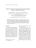
Fig.1showsthesketchoftheexperimentand
wave gauge location for water surface
measurement. Five time ‐series data of water
surface elevation were collected for the
comparison.
2.0=
h
A
m 2.7=
B
D
m 2.2=
T
D
m 625.0=
c
h
m 32.0
=
h
B = 30m
L=25m
G1
G6 G9
G16
G22
2.0=
h
A
m 2.7=
B
D
m 2.2=
T
D
m 625.0=
c
h
m 32.0
=
h
2.0=
h
A
m 2.7=
B
D
m 2.2=
T
D
m 625.0=
c
h
m 32.0
=
h
B = 30m
L=25m
G1
G6 G9
G16
G22
Fig.1.Sketchoftheexperiment.
In Fig. 1, the wave gauge G1 is setup for
themeasurementoftheincidentwaves;wave
gauges G6 and G9 are for the waves in the
shoaling area; and the wave gauges G16 and
G22 are respectively, for waves on the right
side and lee side of the island. The
locations
of the five wave gauges are given in Table 1
inrelationwiththecenteroftheisland.
Table1.Locationofwavegauges
Gaugenum.
c
xx
−
(m)
c
y
y− (m)
G1 9.00 2.25
G6 3.60 0.00
G9 2.60 0.00
G16 0.00 2.58
G22‐2.60 0.00
(
c
x ,
c
y
):coordinateofthecenteroftheisland
3.2.Numericalsimulationanddiscussion
Inthenumericalsimulation,acomputation
domain is setup similar to the experiment.
Themeshisregularwithgridsizeof0.1min
both x and
y
directions.Atfoursidesofthe
computation domain, radiation boundary
conditions are used in order to allow waves
to go freely through the side boundary. A
solitary wave is generated as the initial
conditionatalineparallelwiththe
y
direction,
andlocatedatthedistanceof12.96mfromthe
center of the island. The Manning coefficient
is set to be constant n = 0.016. The initial
solitary wave is created by using the
followingequation:
()
2
3
3
() sech
4
s
A
xA xx
h
⎡
⎤
η= −
⎢
⎥
⎣
⎦
(11)
()
()
g
ux x
h
=η (12)
where
s
x isthecenterofthesolitarywave.
The numerical results of water surface
elevation at five wave‐gauge locations and
runup height on the island are recorded for
PhungDangHieu/VNU JournalofScience,EarthSciences24(2008 ) 79‐86
83
validationofthesimulation.Fig.2ashowsthe
time profile of water surface elevation at the
wave gauge G1. In this figure, it is seen that
the incident solitary wave simulated by the
modelagreesverywellwiththeexperimental
data.Thisgivesusaconfidenceincomparison
oftimeseries
ofwatersurfaceelevationatother
locations in the computation do main, as well
asincomparisonofwaverunupontheisland.
In the Fig. 2b and 2c, at the wave gauges
G6andG9,it isseenthatthesolitarywaveis
well simulated on the shoaling region, the
wave comes to the location after about 4
seconds from the initial time. At first, the
numerical results and experimental data
agree very
well, after that, there are some
discrepancy appeared. This deflection can be
explained due to the reflection from the side
boundariesintheexperi ment donebyBriggs
etal,muchlargerthanthatinthesimulation.
-0.05
0
0.05
0.1
0 5 10 15 20
Time (sec)
Num. NSW Model
Num. Bouss Model
Exp. Data (Briggs et al, 1995)
gauge 1
-0.05
0
0.05
0.1
0 5 10 15 20
Time (sec)
Num. NSW Model
Num. Bouss Model
Exp. Data (Briggs et al, 1995)
gauge 6
-0.05
0
0.05
0.1
0 5 10 15 20
Time (sec)
Num. NSW Model
Num. Bouss Model
Exp. Data (Briggs et al, 1995)
gauge 9
Fig.2.ComparisonofwatersurfaceelevationatlocationsG1,G6,G9:solidthinline:simulatedbycommon
shallowwaterequation;solidthickline:simulatedbyaddingBoussinesqtermtotheshallowwaterequation.
a)
b)
c)
PhungDangHieu/VNU JournalofScience,EarthSciences24(2008 ) 79‐86
84
-0.05
0
0.05
0.1
0 5 10 15 20
Time (sec)
Num. NSW Model
Num. Bouss Model
Exp. Data (Briggs et al, 1995)
gauge 16
-0.05
0
0.05
0.1
0 5 10 15 20
Time (sec)
Num. NSW Model
Num. Bouss Model
Exp. Data (Briggs et al, 1995)
gauge 22
Fig.3.ComparisonofwatersurfaceelevationatlocationsG16andG22:solidthinline:simulatedbycommon
shallowwaterequation;solidthickline:simulatedbyaddingBoussinesqtermtotheshallowwaterequation.
It can be confirmed from the figure that,
thenumericalresultsverysoonbecomestable
having non‐fluctuation when the wave goes
freely out of the experiment domain.
Inversely, the experimental data have a long
tailofdisturbanceandcouldnotbecalmafter
20s (see Fig. 2, at wave gauges
G6 and G9;
andFig3,atwavegaugesG16andG22).This
fluctuation is due to the wave energy
dissipation not enough at the sides of the
experiment basin. However, the form and
height of the arriving solitary wave at all
locations are well matched between
experimental and numerical
results. This is
very important to allow later comparison of
waverunupontheisland.
FromFig. 2andFig.3,itisalsoseenthat,
the wave height at the lee side (gauge G22,
Fig. 3b) of the island is still very high in
comparison with the height at the
front side
(gauge G6, G9, Fig. 2b, 2c) of the island, and
muchbiggerthanthatattherightside(gauge
G16, Fig. 3a) of the island. These results give
us a confidence in confirming that the wave
height at lee side of an circular island can be
large also.
In Fig. 2 and Fig. 3, two sets of
numerical results are plotted. One is
simulatedbythecommonnon‐linearshallow
water equation (NSW), and the other is
simulated by adding the Boussinesq
dispersion term [8] into the NSW. From the
figures, it is confirmed that the model using
the
Boussinesq approximation can give
simulated results much better than the
common NSW based model. Thus, for the
practical purpose of simulation non ‐linear
long wave problem, the Boussinesq
approximationtermsshouldbeconsidered.
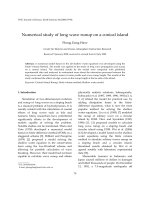
Fig.4showsthesnapshotofwatersurface
displacementonthecomputationdomain.From
the figure, we
can see th at, after the solitary
wavecomestotheisland,thewaverefraction
appears due to the variation of water depth.
Behindtheisland,theedgewavescomefrom
twosidesoftheislandduetowavesbending
around the island and matching together at
a)
b)
PhungDangHieu/VNU JournalofScience,EarthSciences24(2008 ) 79‐86
85
the leeside of the island. Then, they form an
area of very high wave rushing up to the lee
side coast of the island. This mechanism can
be explained for the unexpectedly large
runup heights on the leeside of the Babi and
OkushiriIslandsduetothetsunami.
Fig. 5 is
the comparison of wave runup
around the island, between numerical
simulation and experiment. The horizontal
axisinthefigureindicatestheanglebetween
thelinedrawingfromthecenteroftheisland
tothepointofrunupmeasurementandthey
direction. The angle of 0 degree means that
the
measuringpointisattherightsideofthe
island and on the line through the center of
the island and normal to the incident wave
direction(i.e.paralleltotheydirection).Itis
shown from the figure that, the runup is
highest at the foreside of the island, the
maximum simulated runup height is
somewhatlessthanexperimentaldata.Atthe
leeside of the island, there is an area with
runup higher than both sides of the island.
Thenumericalresultsofrunupheightinthis
area are also smaller than experimental data.
These might be due to the
fact that the
computational mesh not fine enough to
capturehighlynon‐linearinteractionsofedge
wavesattheleeside.Inoverall,thenumerical
model can simulate well the runup height at
manylocationsaroundtheisland. Especially,
the tendency of the runup variation and
runup location are well simulated by
the
present numerical model. This means that,
themodeldevelopedinthisstudyhaspotential
features to apply to the study of practical
problems related with long waves, such as
inundationoftsunamioncoastalareas.
Fig.4.Snapshotsofthewatersurfacedisplacementduetothesolitarywave.
0
0.05
0.1
0.15
0.2
0 50 100 150 200 250 300 350
Angle (deg)
Runup (m).
Num. Result
Exp. data (Briggs et al, 1995)
Fig.5.Runupofwateraroundtheislandduetothesolitarywave(270deg.:atforesideinthenormal
directionofwavepropagation;90deg.:attheleesideoftheisland;0deg.:attherightsideoftheisland;
and180deg.:attheleftsideofthe
island).
PhungDangHieu/VNU JournalofScience,EarthSciences24(2008 ) 79‐86
86
4.Conclusions
A 2D numerical model based on the
shallowwaterequationhasbeensuccessfully
developed for the simulation of long wave
propagation, deformation and runup on the
conical island. The numerical results
simulatedbyNSWmodelandbyBoussinesq
model revealed that by adding Boussinesq
termstotheNSWmodel,simulatedresults
of
long wave propagation and deformation can
be significantly improved. Therefore, it is
worth to mention that Boussinesq
approximation should be considered in a
practical problem related with long waves.
The model also has potential features to
apply to the study of practical problems
related to long waves, su ch as
inundation of
tsunamioncoastalareas.
Simulated results in this study also
confirmthattheareabehindanislandcanbe
attacked by big waves coming from the
opposite side of the island due to non‐linear
interaction of edge waves resulted from
refractionprocesses.
Acknowledgments
This paper was completed within the
framework of Fundamental Research Project
304006 funded by Vietnam Ministry of
ScienceandTechnology.
References
[1] M.J. Briggs et al, Laboratory experiments of
tsunamirunuponacircularisland,PureApplied
Geophys.144(1995)569.
[2] S.Hibbert,D.H.Peregrine,Surfand runupona
beach:auniformbore,JournalofFluidMechanics
95(1979)323.
[3] N.Kobayashi,A.K.Otta,I.Roy,Wavereflection
and
runup on rough slopes, J.Waterway, Port,
CoastalandOceanEngineering113(1987)282.
[4] N.Kobayashi,G.S.DeSilva,K.D.Wattson,Wave
transformation and swashoscillationsongentle
and steep slopes, Journal of Geophysics Research
94(1989)951.
[5] N. Kobayashi, D.T. Cox, A. Wurjanto, Irregular
wavereflectionandrunup
onroughimp ermeable
slopes, Journal of Waterway, Port, Coastal and
OceanEngineering116(1990)708.
[6] N. Kobayashi, A. Wurjanto, Irregular wave
setup and runup on beaches, Journal Waterway,
Port, Coastal and Ocean Engineering 118 (1992)
368.
[7] P.L‐F Liu et al, Runup of solitary wave on a
circular
island, Journal of Fluid Mechanics 302
(1995)259.
[8] P.A.Madsen,O.R.Sorensen,H.A.Schaffer,Surf
zone dynamics simulated by Boussinesq type
model,PartI:Modeldescriptionandcross‐shore
motion of regular waves, Coastal Engineering 32
(1997)255.
[9] N. Shuto, C. Goto, Numerical simulation of
tsunamirunup,CoastalEngineering
Journal‐Japan
21(1978)13.
[10] G. Strang, On the construction and comparison
of difference schemes, SIAM (Soc. Int. Appl.
Math.)JournalofNumericalAnalysis5(1968)506.
[11] V.V.Titov,C.E.Synolakis,Modelingofbreaking
and non‐breaking long‐wave evolution and
runup using VTCS‐2, Journal of Waterway,
Port,
CoastalandOceanEngineering121(1995)308.
[12] V.V. Titov, C.E. Synolakis, Numerical modeling
of tidal wave runup, Journal of Waterway, Port,
CoastalandOceanEngineering124(1998)157.
[13] Y. Wei, X.Z. Mao, K.F. Cheung, Well‐balanced
finite‐volume model for long‐wave runup.
Journal of Waterway, Port, Coastal
and Ocean
Engineering132(2006)114.