Đề tài " On the Julia set of a typical quadratic polynomial with a Siegel disk " ppt
Bạn đang xem bản rút gọn của tài liệu. Xem và tải ngay bản đầy đủ của tài liệu tại đây (2.73 MB, 53 trang )
Annals of Mathematics
On the Julia set of a typical
quadratic polynomial with a
Siegel disk
By C. L. Petersen and S. Zakeri
Annals of Mathematics, 159 (2004), 1–52
On the Julia set of a typical
quadratic polynomial with a Siegel disk
By C. L. Petersen and S. Zakeri
To the memory of Michael R. Herman (1942–2000)
Abstract
Let 0 <θ<1 be an irrational number with continued fraction expansion
θ =[a
1
,a
2
,a
3
, ], and consider the quadratic polynomial P
θ
: z → e
2πiθ
z +
z
2
. By performing a trans-quasiconformal surgery on an associated Blaschke
product model, we prove that if
log a
n
= O(
√
n)asn →∞,
then the Julia set of P
θ
is locally connected and has Lebesgue measure zero.
In particular, it follows that for almost every 0 <θ<1, the quadratic P
θ
has
a Siegel disk whose boundary is a Jordan curve passing through the critical
point of P
θ
. By standard renormalization theory, these results generalize to
the quadratics which have Siegel disks of higher periods.
Contents
1. Introduction
2. Preliminaries
3. A Blaschke model
4. Puzzle pieces and a priori area estimates
5. Proofs of Theorems A and B
6. Appendix: A proof of Theorem C
References
1. Introduction
Consider the quadratic polynomial P
θ
: z → e
2πiθ
z + z
2
, where 0 <θ<1
is an irrational number. It has an indifferent fixed point at 0 with multiplier
P
θ
(0) = e
2πiθ
, and a unique finite critical point located at −e
2πiθ
/2. Let A
θ
(∞)
be the basin of attraction of infinity, K
θ
= C A
θ
(∞) be the filled Julia set,
2 C. L. PETERSEN AND S. ZAKERI
and J
θ
= ∂K
θ
be the Julia set of P
θ
. The behavior of the sequence of iterates
{P
◦n
θ
}
n≥0
near J
θ
is intricate and highly nontrivial. (For a comprehensive
account of iteration theory of rational maps, we refer to [CG] or [M].)
The quadratic polynomial P
θ
is said to be stable near the indifferent fixed
point 0 if the family of iterates {P
◦n
θ
}
n≥0
restricted to a neighborhood of 0 is
normal in the sense of Montel. In this case, the largest neighborhood of 0 with
this property is a simply connected domain ∆
θ
called the (maximal) Siegel disk
of P
θ
. The unique conformal isomorphism ψ
θ
:∆
θ
−→ D with ψ
θ
(0) = 0 and
ψ
θ
(0) > 0 linearizes P
θ
in the sense that ψ
θ
◦ P
θ
◦ ψ
−1
θ
(z)=R
θ
(z):=e
2πiθ
z
on
D.
Consider the continued fraction expansion θ =[a
1
,a
2
,a
3
, ] with a
n
∈
N,
and the rational convergents p
n
/q
n
:= [a
1
,a
2
, ,a
n
]. The number θ is said
to be of bounded type if {a
n
} is a bounded sequence. A celebrated theorem of
Brjuno and Yoccoz [Yo3] states that the quadratic polynomial P
θ
has a Siegel
disk around 0 if and only if θ satisfies the condition
∞
n=1
log q
n+1
q
n
< +∞,
which holds almost everywhere in [0, 1]. But this theorem gives no information
as to what the global dynamics of P
θ
should look like. The main result of this
paper is a precise picture of the dynamics of P
θ
for almost every irrational θ
satisfying the above Brjuno-Yoccoz condition:
Theorem A. Let E denote the set of irrational numbers θ =[a
1
,a
2
,a
3
, ]
which satisfy the arithmetical condition
log a
n
= O(
√
n) as n →∞.
If θ ∈E, then the Julia set J
θ
is locally connected and has Lebesgue measure
zero. In particular, the Siegel disk ∆
θ
is a Jordan domain whose boundary
contains the finite critical point.
This theorem is a rather far-reaching generalization of a theorem which
proves the same result under the much stronger assumption that θ is of bounded
type [P2]. It is immediate from the definition that the class E contains all ir-
rationals of bounded type. But the distinction between the two arithmetical
classes is far more remarkable, since E has full measure in [0, 1] whereas num-
bers of bounded type form a set of measure zero (compare Corollary 2.2).
The foundations of Theorem A was laid in 1986 by several people, notably
Douady [Do]. Their idea was to construct a model map F
θ
for P
θ
by performing
surgery on a cubic Blaschke product f
θ
. Along with the surgery, they also
proved a meta theorem asserting that F
θ
and P
θ
are quasiconformally conjugate
if and only if f
θ
is quasisymmetrically conjugate to the rigid rotation R
θ
on S
1
.
QUADRATIC POLYNOMIALS WITH A SIEGEL DISK 3
Soon after, Herman used a cross ratio distortion inequality of
´
Swiatek [Sw] for
critical circle maps to give this meta theorem a real content. He proved that f
θ
(or any real-analytic critical circle map with rotation number θ for that matter)
is quasisymmetrically conjugate to R
θ
if and only if θ is of bounded type [H2].
In 1993, Petersen showed that the “Julia set” J(F
θ
) is locally connected for
every irrational θ, and has measure zero for every θ of bounded type [P2]. The
measure zero statement was soon extended by Lyubich to all irrational θ.It
follows from Herman’s theorem that J
θ
is locally connected and has measure
zero when θ is of bounded type. In this case, the Siegel disk ∆
θ
is a quasidisk
in the sense of Ahlfors and its boundary contains the finite critical point.
The idea behind the proof of Theorem A is to replace the technique of
quasiconformal surgery by a trans-quasiconformal surgery on a cubic Blaschke
product f
θ
. Let us give a brief sketch of this process.
We fix an irrational number 0 <θ<1 and following [Do] we consider the
degree 3 Blaschke product
f
θ
: z → e
2πit
z
2
z − 3
1 − 3z
,
which has a double critical point at z = 1. Here 0 <t= t(θ) < 1 is the unique
parameter for which the critical circle map f
θ
|
S
1
: S
1
→ S
1
has rotation number
θ (see subsection 2.4). By a theorem of Yoccoz [Yo1], there exists a unique
homeomorphism h
θ
: S
1
→ S
1
with h
θ
(1) = 1 such that h
θ
◦ f
θ
|
S
1
= R
θ
◦ h
θ
.
Let H :
D → D be any homeomorphic extension of h
θ
and define
F
θ
(z)=F
θ,H
(z):=
f
θ
(z)if|z|≥1
(H
−1
◦ R
θ
◦ H)(z)if|z| < 1.
Then F
θ
is a degree 2 topological branched covering of the sphere. It is holo-
morphic outside of
D and is topologically conjugate to the rigid rotation R
θ
on D. This is the candidate model for the quadratic map P
θ
.
By way of comparison, if there is any correspondence between P
θ
and F
θ
,
the Siegel disk for P
θ
should correspond to the unit disk for F
θ
, while the
other bounded Fatou components of P
θ
should correspond to other iterated
F
θ
-preimages of the unit disk, which we call drops. The basin of attraction
of infinity for P
θ
should correspond to a similar basin A(∞) for F
θ
(which is
the immediate basin of attraction of infinity for f
θ
). By imitating the case
of polynomials, we define the “filled Julia set” K(F
θ
)asC A(∞) and the
“Julia set” J(F
θ
) as the topological boundary of K(F
θ
), both of which are
independent of the homeomorphism H (compare Figure 2).
By the results of Petersen and Lyubich mentioned above, J(F
θ
) is locally
connected and has measure zero for all irrational numbers θ. Thus, the local-
connectivity statement in Theorem A will follow once we prove that for θ ∈E
there exists a homeomorphism ϕ
θ
: C → C such that ϕ
θ
◦ F
θ
◦ ϕ
−1
θ
= P
θ
.
4 C. L. PETERSEN AND S. ZAKERI
The measure zero statement in Theorem A will follow once we prove ϕ
θ
is
absolutely continuous.
The basic idea described by Douady in [Do] is to choose the homeomorphic
extension H in the definition of F
θ
to be quasiconformal, which by Herman’s
theorem is possible if and only if θ is of bounded type. Taking the Beltrami
differential of H on
D
, and spreading it by the iterated inverse branches of
F
θ
to all the drops, one obtains an F
θ
-invariant Beltrami differential µ on
C
with bounded dilatation and with the support contained in the filled Julia
set K(F
θ
). The measurable Riemann mapping theorem shows that µ can be
integrated by a quasiconformal homeomorphism which, when appropriately
normalized, yields the desired conjugacy ϕ
θ
.
To go beyond the bounded type class in the surgery construction, one has
to give up the idea of a quasiconformal surgery. The main idea, which we
bring to work here, is to use extensions H which are trans-quasiconformal, i.e.,
have unbounded dilatation with controlled growth. What gives this approach
a chance to succeed is the theorem of David on integrability of certain Beltrami
differentials with unbounded dilatation [Da]. David’s integrability condition
requires that for all large K, the area of the set of points where the dilatation
is greater than K be dominated by an exponentially decreasing function of K
(see subsection 2.5 for precise definitions). An orientation-preserving homeo-
morphism between planar domains is a David homeomorphism if it belongs to
the Sobolev class W
1,1
loc
and its Beltrami differential satisfies the above integra-
bility condition. Such homeomorphisms are known to preserve the Lebesgue
measure class.
To carry out a trans-quasiconformal surgery, we have to address two fun-
damental questions:
Question 1. Under what optimal arithmetical condition E
DE
on θ does
the linearization h
θ
admit a David extension H : D
→
D
?
Question 2. Under what optimal arithmetical condition E
DI
on θ does
the model F
θ
admit an invariant Beltrami differential satisfying David’s inte-
grability condition in the plane?
It turns out that the two questions have the same answer, i.e., E
DE
= E
DI
.
Clearly E
DE
⊇E
DI
, but the other inclusion is a nontrivial result, which we
prove in this paper by means of the following construction.
Define a measure ν supported on
D by summing up the push forward of
Lebesgue measure on all the drops. In other words, for any measurable set
E ⊂
D, set
ν(E) := area(E)+
g
area(g(E)),
QUADRATIC POLYNOMIALS WITH A SIEGEL DISK 5
where the summation is over all the univalent branches g = F
−k
θ
mapping D to
various drops. Evidently ν is absolutely continuous with respect to Lebesgue
measure on
D. However, we prove a much sharper result:
Theorem B. The measure ν is dominated by a universal power of Lebesgue
measure. In other words, there exist a universal constant 0 <β<1 and a con-
stant C>0(depending on θ) such that
ν(E) ≤ C (area(E))
β
for every measurable set E ⊂
D.
It follows immediately from this key estimate that the F
θ
-invariant Bel-
trami differential µ constructed above satisfies David’s integrability condition
if µ|
D
does, or equivalently, if there is a David extension H for h
θ
.
Theorem B can be used to prove that a conjugacy ϕ
θ
between F
θ
and
P
θ
exists whenever h
θ
admits a David extension to the disk. The following
theorem proves the existence of David extensions for circle homeomorphisms
which arise as linearizations of critical circle maps with rotation numbers in E.
This theorem, as formulated here in the context of our trans-quasiconformal
surgery, is new. However, we should emphasize that all the main ingredients
of its constructive proof are already present in a manuscript of Yoccoz [Yo2].
Theorem C. Let f :
S
1
→ S
1
be a critical circle map whose rotation
number θ =[a
1
,a
2
,a
3
, ] belongs to the arithmetical class E. Then the nor-
malized linearizing map h :
S
1
→ S
1
, which satisfies h ◦ f = R
θ
◦ h, admits a
David extension H :
D
→
D
so that
area
z ∈ D :
∂H(z)
∂H(z)
> 1 −ε
≤ Me
−
α
ε
for all 0 <ε<ε
0
.
Here M>0 is a universal constant, while in general the constant α>0
depends on lim sup
n→∞
(log a
n
)/
√
n and the constant 0 <ε
0
< 1 depends on f .
Let us point out that Theorem C proves E⊂E
DE
, where E
DE
is the
arithmetical condition in Question 1. We have reasons to suspect that the
above inclusion might in fact be an equality, but so far we have not been able
to prove this.
When θ is of bounded type, the boundary of the Siegel disk ∆
θ
is a
quasicircle, so it clearly has Hausdorff dimension less than 2. McMullen has
proved that in this case the entire Julia set J
θ
has Hausdorff dimension less
than 2 [Mc2], a result which improves the measure zero statement in Petersen’s
theorem. The situation when θ belongs to E but is not of bounded type
might be quite different. In this case, the proof of Theorem A shows that
the boundary of ∆
θ
is a David circle, i.e., the image of the round circle under
a David homeomorphism. It can be shown that, unlike quasiconformal maps,
6 C. L. PETERSEN AND S. ZAKERI
David homeomorphisms do not preserve sets of Hausdorff dimension 0 or 2,
and in fact there are David circles of Hausdorff dimension 2 [Z2]. So, a priori,
the boundary of ∆
θ
might have Hausdorff dimension 2 as well. Motivated by
these remarks, we ask:
Question 3. What can be said about the Hausdorff dimension of J
θ
when
θ belongs to E but is not of bounded type? Does there exist such a θ for which
J
θ
,oreven∂∆
θ
, has Hausdorff dimension 2?
The use of trans-quasiconformal surgery in holomorphic dynamics was
pioneered by Ha¨ıssinsky who showed how to produce a parabolic point from a
pair of attracting and repelling points when the repelling point is not in the
ω-limit set of a recurrent critical point [Ha]. In contrast, our maps have a
recurrent critical point whose orbit is dense in the boundary of the disk on
which we perform surgery.
The idea of constructing rational maps by quasiconformal surgery on
Blaschke products has been taken up by several authors; for instance Zakeri,
who in [Z1] models the one-dimensional parameter space of cubic polynomials
with a Siegel disk of a given bounded type rotation number. Also this idea is
central to the work of Yampolsky and Zakeri in [YZ], where they show that
any two quadratic Siegel polynomials P
θ
1
and P
θ
2
with bounded type rotation
numbers θ
1
and θ
2
are mateable provided that θ
1
=1− θ
2
. We believe adap-
tations of the ideas and techniques developed in the present paper will give
generalizations of those results to rotation numbers in E.
Acknowledgements. The first author would like to thank the Mathematics
Department of Cornell University for its hospitality and IMFUA at Roskilde
University for its financial support. The second author is grateful to IMS at
Stony Brook for supporting part of this research through NSF grant DMS
9803242 during the spring semester of 1999. Further thanks are due to the
referee whose suggestions improved our presentation of puzzle pieces in Section
4, and to P. Ha¨ıssinsky whose comment prompted us to add Lemma 5.5 to
our early version of this paper.
2. Preliminaries
2.1. General notation. We will adopt the following notation throughout
this paper:
•
T is the quotient R/Z.
•
S
1
is the unit circle {z ∈ C : |z| =1}; we often identify T and S
1
via the
exponential map x → e
2πix
without explicitly mentioning it.
QUADRATIC POLYNOMIALS WITH A SIEGEL DISK 7
•|I| is the Euclidean length of a rectifiable arc I ⊂
C.
• For x, y ∈
T or S
1
which are not antipodal, [x, y]=[y, x] (resp. ]x, y[=
]y, x[) denotes the shorter closed (resp. open) interval with endpoints x, y.
• diam(·), dist(·, ·) and area(·) denote the Euclidean diameter, Euclidean
distance and Lebesgue measure in
C.
• For a hyperbolic Riemann surface X,
X
(·), diam
X
(·) and dist
X
(·) denote
the hyperbolic arclength, diameter and distance in X.
• In a given statement, by a universal constant we mean one which is inde-
pendent of all the parameters/variables involved. Two positive numbers
a, b are said to be comparable up to a constant C>1ifb/C ≤ a ≤ bC.
For two positive sequences {a
n
} and {b
n
}, we write a
n
b
n
if there ex-
ists a universal constant C>1 such that a
n
≤ Cb
n
for all large n.We
define a
n
b
n
in a similar way. We write a
n
b
n
if b
n
a
n
b
n
, i.e., if
there exists a universal constant C>1 such that b
n
/C ≤ a
n
≤ Cb
n
for
all large n. Any such relation will be called an asymptotically universal
bound. Note that for any such bound, the corresponding inequalities hold
for every n if C is replaced by a larger constant (which may well depend
on our sequences and no longer be universal).
Another way of expressing an asymptotically universal bound, which we
will often use, is as follows: When a
n
b
n
, we say that a
n
/b
n
is bounded
from above by a constant which is asymptotically universal. Similarly,
when a
n
b
n
, we say that a
n
and b
n
are comparable up to a constant
which is asymptotically universal.
Finally, let {a
n
= a
n
(x)} and {b
n
= b
n
(x)} depend on a parameter x
belonging to a set X. Then we say that a
n
b
n
uniformly in x ∈ X if
there exists a universal constant C>1 and an integer N ≥ 1 such that
b
n
(x)/C ≤ a
n
(x) ≤ Cb
n
(x) for all n ≥ N and all x ∈ X.
2.2. Some arithmetic. Here we collect some basic facts about continued
fractions; see [Kh] or [La] for more details. Let 0 <θ<1 be an irrational
number and consider the continued fraction expansion
θ =
1
a
1
+
1
a
2
+
1
a
3
+ ···
=[a
1
,a
2
,a
3
, ],
with a
n
= a
n
(θ) ∈ N. The n-th convergent of θ is the irreducible fraction
p
n
/q
n
:= [a
1
,a
2
, ,a
n
]. We set p
0
:= 0, q
0
:= 1. It is easy to verify the
recursive relations
(2.1) p
n
= a
n
p
n−1
+ p
n−2
and q
n
= a
n
q
n−1
+ q
n−2
8 C. L. PETERSEN AND S. ZAKERI
for n ≥ 2. The denominators q
n
grow exponentially fast; in fact it follows
easily from (2.1) that
q
n
≥ (
√
2)
n
for n ≥ 2.
Elementary arithmetic shows that
(2.2)
1
q
n
(q
n
+ q
n+1
)
<
θ −
p
n
q
n
<
1
q
n
q
n+1
,
which implies p
n
/q
n
→ θ exponentially fast.
Various arithmetical conditions on irrational numbers come up in the
study of indifferent fixed points of holomorphic maps. Of particular interest
are:
• The class D
d
of Diophantine numbers of exponent d ≥ 2. An irrational θ
belongs to D
d
if there exists some C>0 such that |θ − p/q|≥Cq
−d
for
all rationals p/q. It follows immediately from (2.2) that for any d ≥ 2
(2.3) θ ∈D
d
⇔ sup
n
q
n+1
q
n
d−1
< +∞⇔sup
n
a
n+1
q
n
d−2
< +∞.
• The class D :=
d≥2
D
d
of Diophantine numbers. From (2.3) it follows
that
θ ∈D⇔sup
n
log q
n+1
log q
n
< +∞.
• The class D
2
of Diophantine numbers of exponent 2. Again by (2.3)
θ ∈D
2
⇔ sup
n
a
n
< +∞.
For this reason, any such θ is called a number of bounded type.
• The class B of numbers of Brjuno type. By definition,
θ ∈B⇔
∞
n=1
log q
n+1
q
n
< +∞.
We have the proper inclusions
D
2
D
d
D B
for any d>2. Diophantine numbers of any exponent d>2 have full measure
in [0, 1] while numbers of bounded type form a set of measure zero.
The following theorem characterizes the asymptotic growth of the se-
quence {a
n
} for random irrational numbers:
QUADRATIC POLYNOMIALS WITH A SIEGEL DISK 9
Theorem 2.1. Let ψ :
N → R be a given positive function.
(i) If
∞
n=1
1
ψ(n)
< +∞, then for almost every irrational 0 <θ<1 there are
only finitely many n for which a
n
(θ) ≥ ψ(n).
(ii) If
∞
n=1
1
ψ(n)
=+∞, then for almost every irrational 0 <θ<1 there are
infinitely many n for which a
n
(θ) ≥ ψ(n).
This theorem is often attributed to E. Borel and F. Bernstein, at least in
the case ψ is increasing. For a proof of the general case, see Khinchin’s book
[Kh].
Corollary 2.2. Let E be the set of all irrational numbers 0 <θ<1 for
which the sequence {a
n
= a
n
(θ)} satisfies
(2.4) log a
n
= O(
√
n) as n →∞.
Then E has full measure in [0, 1].
The class E will be the center of focus in the present paper. It is easily
seen to be a proper subclass of D
d
for any d>2.
2.3. Rigid rotations. We now turn to elementary properties of rigid rota-
tions on the circle. For a comprehensive treatment, we recommend Herman’s
monograph [H1]. Let R
θ
: x → x + θ (mod Z) denote the rigid rotation by the
irrational number θ.Forx ∈
R, set x := inf
n∈Z
|x − n|. Then, for n ≥ 2,
q
n
θ < iθ for all 1 ≤ i<q
n
.
Thus, considering the orbit of 0 ∈
T under the iteration of R
θ
, the denominators
q
n
constitute the moments of closest return. Clearly the same is true for the
orbit of every point. It is not hard to verify that
(2.5) q
n
θ =(−1)
n
(q
n
θ −p
n
),
so that the closest returns occur alternately on the left and right sides of 0.
Consider the decreasing sequence q
1
θ > q
2
θ > q
3
θ > ··· and define
the scaling ratio
s
n
:=
q
n
θ
q
n+1
θ
> 1.
By (2.1) and (2.5)
s
n−1
= a
n+1
+
1
s
n
.
In particular, the two sequences {a
n+2
} and {s
n
} have the same asymptotic
behavior. For example, it follows that the sequence {s
n
} is bounded if and
only if θ is of bounded type.
There are two basic facts about the structure of the orbits of rotations
that we will use repeatedly:
10 C. L. PETERSEN AND S. ZAKERI
• For i ∈ Z, let x
i
denote the iterate R
−i
θ
(0) (Caution: We have labelled
the orbit of 0 backwards to simplify the subsequent notations; this cor-
responds to the standard notation for the inverse map R
−1
θ
). Given two
consecutive closest return moments q
n
and q
n+1
, the points in the orbit
of 0 occur in the order shown in Figure 1 (the picture shows the case n is
odd; for the case n is even simply rotate the picture 180
◦
about 0). Note
that |[0,x
q
n
]| = |[0,x
−q
n
]| = q
n
θ. Evidently, the orbit of any other
point of
T enjoys the same order.
x
q
n
+1
x
q
n
+1
q
n
q
n
-1
x
q
n
+
x
q
n
-1
0
n
q
x
x
q
n
+1
Figure 1. Selected points in the orbit of 0 under the rigid rotation.
• Let I
n
:= [0,x
q
n
]bethen-th closest return interval for 0. Then the
collection of intervals
(2.6) Π
n
(R
θ
):={R
−i
θ
(I
n
)}
0≤i≤q
n+1
−1
∪{R
−i
θ
(I
n+1
)}
0≤i≤q
n
−1
defines a partition of the circle modulo the common endpoints. We call
Π
n
(R
θ
) the dynamical partition of level n for R
θ
.
Theorem 2.3 (Poincar´e). Let f :
T → T be any circle homeomorphism
without periodic points. Then there exists a unique irrational number θ and a
continuous degree 1 monotone map h :
T → T such that h ◦ f = R
θ
◦ h.
The number θ is called the rotation number of f and is denoted by ρ(f).
The map h is called a Poincar´e semiconjugacy. It easily follows from this
theorem that the combinatorial structure of the orbits of any circle homeo-
morphism with irrational rotation number θ is the same as the combinatorial
structure of the orbit of 0 for R
θ
.
2.4. Critical circle maps. For our purposes, a critical circle map will be
a real-analytic homeomorphism of
T with a critical point at 0. It was proved
by Yoccoz [Yo1] that for a critical circle map with irrational rotation number,
every Poincar´e semiconjugacy is in fact a conjugacy:
Theorem 2.4 (Yoccoz). Let f :
T → T be a critical circle map with
irrational rotation number ρ(f)=θ. Then there exists a homeomorphism
h :
T → T such that h ◦ f = R
θ
◦ h. This h is uniquely determined once
normalized by h(0) = 0.
We will reserve the notation x
i
for the backward iterate f
−i
(0) of the
critical point 0 and I
n
:= [0,x
q
n
] for the n-th closest return interval under f
−1
.
QUADRATIC POLYNOMIALS WITH A SIEGEL DISK 11
The dynamical partition Π
n
(f) of level n for f will be defined as h
−1
(Π
n
(R
θ
)),
or equivalently, by (2.6) with R
θ
replaced by f.
Herman took the next step in studying critical circle maps by showing
that the linearizing map h is quasisymmetric if and only if ρ(f) is irrational of
bounded type. The proof of this theorem makes essential use of the existence
of real a priori bounds developed by
´
Swiatek and Herman. Here is a version of
their result needed in this paper (see [Sw], [H2], [dFdM], or [P4]).
Theorem 2.5 (
´
Swiatek-Herman). Let f :
T → T
be a critical circle map
with ρ(f) irrational. Then
(i) There exists an asymptotically universal bound
|[y, f
◦q
n
(y)]||[y,f
−q
n
(y)]|
which holds uniformly in y ∈
T.
(ii) The lengths of any two adjacent intervals in the dynamical partition
Π
n
(f) are comparable up to a bound which is asymptotically universal.
In other words,
max
|I|
|J|
: I,J ∈ Π
n
(f) are adjacent
1.
An important corollary of (ii), which exhibits a sharp contrast with the
case of rigid rotations, is that the scaling ratio is bounded from above and
below by an asymptotically universal constant regardless of the map f :
s
n
(f):=
|I
n
|
|I
n+1
|
1.
Remark 2.6. The above (i) and (ii) are presumably the most general
statements one can expect when working with the class of all critical circle
maps. However, stronger versions of these bounds can be obtained by restrict-
ing to a special class of such maps. For example, fix a critical circle map f
0
and consider the one-dimensional family
F = {R
t
◦ f
0
:0≤ t ≤ 1 and ρ(R
t
◦ f
0
) is irrational}.
Then, within this family the above bounds hold for all n (rather than all large
n), with the constant depending only on f
0
and not on t. In other words, there
exists a constant C = C(f
0
) > 1 such that
1
C
≤
|[y, f
◦q
n
(y)]|
|[y, f
−q
n
(y)]|
≤ C for all n ≥ 1,y∈
T, and f ∈F,
1
C
≤ max
|I|
|J|
: I,J ∈ Π
n
(f) are adjacent
≤ C for all n ≥ 1 and f ∈F.
12 C. L. PETERSEN AND S. ZAKERI
We will need the following result on the size of the intervals in the dy-
namical partitions for a critical circle map; it is a direct consequence of real
a priori bounds (see for example [dFdM, Th. 3.1]):
Lemma 2.7. Let f :
T → T be a critical circle map, with ρ(f) irrational,
and let Π
n
(f) denote the dynamical partition of level n for f. Then there exist
universal constants 0 <σ
1
<σ
2
< 1 such that
σ
n
1
|I
n
|≤ max
I∈Π
n
(f)
|I|
σ
n
2
.
2.5. David homeomorphisms. An orientation-preserving homeomorphism
ϕ :Ω→ Ω
between planar domains belongs to the Sobolev class W
1,1
loc
(Ω) if
the distributional partial derivatives ∂ϕ and
∂ϕ exist and are locally integrable
in Ω (equivalently, if ϕ is absolutely continuous on lines in Ω; see for example
[A]). In this case, ϕ is differentiable almost everywhere and the Jacobian
Jac(ϕ)=|∂ϕ|
2
−|∂ϕ|
2
≥ 0 is locally integrable.
A Beltrami differential in Ω is a measurable (−1, 1)-form µ = µ(z) d
z/dz
such that |µ| < 1 almost everywhere in Ω. We say that µ is integrable if there is
a homeomorphism ϕ :Ω→ Ω
in W
1,1
loc
(Ω) which solves the Beltrami equation
∂ϕ = µ∂ϕ. The classical quasiconformal mappings arise as the solutions of
the Beltrami equation in the case µ
∞
< 1. However, there are numerous
important problems in which one has to study this equation when µ
∞
=1.
Simple examples show that such a µ is not generally integrable, so one has to
seek conditions on the growth of |µ| which guarantee integrability. One such
condition was given by Guy David in [Da], who studied Beltrami differentials
satisfying an exponential growth condition. Let us call µ a David-Beltrami
differential if there exist constants M>0, α>0, and 0 <ε
0
< 1 such that
(2.7) area{z ∈ Ω:|µ|(z) > 1 − ε}≤Me
−
α
ε
for all 0 <ε<ε
0
.
This notion can be extended to arbitrary domains on the sphere
C; it suffices
to replace the Euclidean area with the spherical area in the growth condition
(2.7).
David proved that the analogue of the measurable Riemann mapping the-
orem [AB] holds for the class of David-Beltrami differentials [Da]:
Theorem 2.8 (David). Let Ω be a domain in
C and µ be a David -
Beltrami differential in Ω. Then µ is integrable. More precisely, there exists an
orientation-preserving homeomorphism ϕ :Ω→ Ω
in W
1,1
loc
(Ω) which satisfies
∂ϕ = µ∂ϕ almost everywhere. Moreover, ϕ is unique up to postcomposition
with a conformal map. In other words, if Φ:Ω→ Ω
is another homeomorphic
solution of the same Beltrami equation in W
1,1
loc
(Ω), then Φ ◦ ϕ
−1
:Ω
→ Ω
is
a conformal map.
QUADRATIC POLYNOMIALS WITH A SIEGEL DISK 13
Solutions of the Beltrami equation given by this theorem are called David
homeomorphisms. They differ from classical quasiconformal maps in many
respects. A significant example is the fact that the inverse of a David home-
omorphism is not necessarily David. However, they enjoy some convenient
properties of quasiconformal maps such as compactness; see [T] for a study of
some of these similarities. The following result is particularly important [Da]:
Theorem 2.9. Let ϕ :Ω→ Ω
be a David homeomorphism. Then ϕ
and ϕ
−1
are both absolutely continuous; in other words, for a measurable set
E ⊂ Ω,
area(E)=0⇐⇒ area(ϕ(E))=0.
It easily follows that if ϕ :Ω→ Ω
is a David homeomorphism, then
∂ϕ = 0 almost everywhere in Ω. Thus, the complex dilatation of ϕ, defined by
the measurable (−1, 1)-form
µ
ϕ
:=
∂ϕ
∂ϕ
d
z
dz
is a well-defined David-Beltrami differential in the sense of (2.7). Equivalently,
the real dilatation of ϕ, given by
K
ϕ
:=
1+|µ
ϕ
|
1 −|µ
ϕ
|
,
satisfies a condition of the form
(2.8) area{z ∈ Ω:K
ϕ
(z) >K}≤Me
−αK
for all K>K
0
for some constants M>0, α>0, and K
0
> 1.
2.6. Extensions of linearizing homeomorphisms. Let f be a critical circle
map with ρ(f) irrational and consider the linearizing map h given by Yoc-
coz’s Theorem 2.4. The problem of extending h to a self-homeomorphism of
the disk with nice analytic properties arises in various circumstances in holo-
morphic dynamics, particularly in the construction of Siegel disks by means
of surgery. When ρ(f) is of bounded type, it follows from Theorem 2.5 that
h is quasisymmetric. Hence, by the theorem of Beurling-Ahlfors [BA], it can
be extended to a quasiconformal map
D → D whose dilatation only depends
on the quasisymmetric norm of h (which in turn only depends on sup
n
a
n
(θ),
where θ = ρ(f)). This allows a quasiconformal surgery (compare [Do], [P2],
[Z1], or [YZ]).
On the other hand, when ρ(f ) is not of bounded type, again by Theo-
rem 2.5, h fails to be quasisymmetric and hence it admits no quasiconformal
extension. Thus, one is forced to give up the idea of quasiconformal surgery.
Still, one can ask if in this case h admits a David extension to
D. One
way to address this problem is to develop a Beurling-Ahlfors theory for David
14 C. L. PETERSEN AND S. ZAKERI
homeomorphisms of the disk. For example, it is possible to show that a circle
homeomorphism whose local distortion has controlled growth admits a David
extension. But, to the best of our knowledge, the problem of characterizing
boundary values of David homeomorphisms has not yet been solved completely:
Problem. Find necessary and sufficient conditions for a circle homeomor-
phism to admit a David extension to the unit disk.
Another approach, less general but very effective in our dynamical frame-
work, is to attempt to construct David extensions directly for the circle home-
omorphisms which arise as linearizing maps of critical circle maps. This ap-
proach turns out to be successful because of the existence of real a priori
bounds (Theorem 2.5). In fact, using Yoccoz’s work in [Yo2], one can prove
the following:
Theorem C. Let f :
S
1
→ S
1
be a critical circle map whose rotation
number θ =[a
1
,a
2
,a
3
, ] belongs to the arithmetical class E defined in (2.4).
Then the linearizing map h :
S
1
→ S
1
, which satisfies h ◦ f = R
θ
◦ h and
h(1) = 1, admits a David extension H :
D → D. Moreover, the constant
M in condition (2.7) is universal, while in general α depends on
lim sup
n→∞
(log a
n
)/
√
n and ε
0
depends on f.
The proof of this result is rather lengthy and will be presented in the
appendix.
3. A Blaschke model
3.1. Definitions. Given an irrational number 0 <θ<1, consider the
degree 3 Blaschke product
(3.1) f = f
θ
: z → e
2πit(θ)
z
2
z − 3
1 − 3z
,
which has superattracting fixed points at 0 and ∞ and a double critical point
at z = 1. Here 0 <t(θ) < 1 is the unique parameter for which the critical circle
map f|
S
1
: S
1
→ S
1
has rotation number θ. By Theorem 2.4, there exists a
unique homeomorphism h :
S
1
→ S
1
with h(1) = 1 such that h ◦f|
S
1
= R
θ
◦h.
Let H :
D → D be any homeomorphic extension of h and define
(3.2) F (z)=F
θ,H
(z):=
f(z)if|z|≥1
(H
−1
◦ R
θ
◦ H)(z)if|z| < 1.
It is easy to see that F is a degree 2 topological branched covering of the
sphere which is holomorphic outside of
D and is topologically conjugate to a
QUADRATIC POLYNOMIALS WITH A SIEGEL DISK 15
rigid rotation on
D. By imitating the polynomial case, we define the “filled
Julia set” of F by
K(F ):={z ∈
C : The orbit {F
◦n
(z)}
n≥0
is bounded}
and the “Julia set” of F as the topological boundary of K(F):
J(F ):=∂K(F ).
Let A(∞) be the basin of attraction of ∞ for F . Then A(∞) is simply-
connected and
K(F )=
C
A(∞),J(F )=∂A(∞).
Let us point out that although the homeomorphism H is by no means canon-
ical, neither J(F ) nor K(F ) nor any of the definitions to follow depends on a
particular choice of H. This is simply because the constructions do not involve
the values of F on
D. The main purpose of introducing F for the following
constructions is to forget about the f -preimages of
D in D. A particular choice
of H is only used in the final step of the proof of Theorem A, where we need
H to be a David homeomorphism.
The Blaschke product f was introduced by Douady and Herman [Do],
using an earlier idea of Ghys, and has been used by various authors in order
to study rational maps with Siegel disks; see for example [P2] and [Mc2] for
the case of quadratic polynomials, and [Z1] and [YZ] for variants in the case
of cubic polynomials and quadratic rational maps.
3.2. Drops and limbs. Here we follow the presentations of [P2] and [YZ]
with minor modifications. The reader might consult either of these references
for a more detailed description.
Figure 2. Filled Julia set K(F ) for θ =[a
1
,a
2
,a
3
, ], where a
n
= e
√
n
.
16 C. L. PETERSEN AND S. ZAKERI
By definition, the unique component of F
−1
(D) D is called the 0-drop
of F and is denoted by U
0
. (In Figure 2, U
0
is the prominently visible Jordan
domain attached to the unit disk at z = 1.) For n ≥ 1, any component U of
F
−n
(U
0
) is a Jordan domain called an n-drop, with n being the depth of U .
The map F
◦n
= f
◦n
: U → U
0
is a conformal isomorphism which extends
isomorphically to a neighborhood of
U, because U
0
does not intersect the
forward orbit of the critical values. The unique point F
−n
(1) ∩ ∂U is called
the root of U and is denoted by x(U ). The boundary ∂U is a real-analytic
Jordan curve except at the root where it has an angle of π/3. We simply refer
to U as a drop when the depth is not important. For convenience, we define
D
tobea(−1)-drop, i.e., a drop of depth −1. Note that these drops do not
depend on the extension H used to define the map F in (3.2).
Let U and V be distinct drops of depths m and n, respectively, with
m ≤ n. Then either
U ∩V = ∅ or else U ∩V = x(V ) and m<n. In the latter
case, we call U the parent of V , and V a child of U. Every n-drop with n ≥ 0
has a unique parent which is an m-drop with −1 ≤ m<n. In particular, the
root of this n-drop belongs to the boundary of its parent.
By definition,
D is said to be of generation 0. Any child of D is of gen-
eration 1. In general, a drop is of generation k if and only if its parent is of
generation k − 1. Given a point w ∈
n≥0
F
−n
(1), there exists a unique drop
U with x(U)=w. In particular, two distinct children of a parent have distinct
roots.
We give a symbolic description of drops by assigning addresses to them.
Set U
∅
:= D, where ∅ is the empty index. For n ≥ 0, let x
n
:= F
−n
(1) ∩ S
1
and let U
n
be the n-drop of generation 1 with root x
n
. Let ι = ι
1
,ι
2
, ,ι
k
be
any multi-index of length k ≥ 1, where each ι
j
is a nonnegative integer. We
recursively define the (ι
1
+ι
2
+···+ι
k
)-drop U
ι
1
,ι
2
, ,ι
k
of generation k with root
x(U
ι
1
,ι
2
, ,ι
k
)=x
ι
1
,ι
2
, ,ι
k
as follows. We have already defined these for k =1.
Suppose that we have defined x
ι
1
,ι
2
, ,ι
k−1
for all multi-indices ι
1
,ι
2
, ,ι
k−1
of
length k −1. Then, we define
x
ι
1
,ι
2
, ,,ι
k
:= F
−(1+ι
1
)
(x
ι
2
, ,ι
k
) ∩ ∂U
ι
1
,ι
2
, ,ι
k−1
.
The drop U
ι
1
,ι
2
, ,ι
k
will be determined by the condition of having x
ι
1
,ι
2
, ,ι
k
as
its root. By the way these drops have been given addresses, we have
F (U
ι
1
,ι
2
, ,ι
k
)=
U
ι
2
, ,ι
k
if ι
1
=0
U
ι
1
−1,ι
2
, ,ι
k
if ι
1
> 0.
Let us fix a drop U
ι
1
, ,ι
k
. By definition, the limb L
ι
1
, ,ι
k
is the closure
of the union of this drop and all its descendants, i.e., children, grandchildren,
etc.:
L
ι
1
, ,ι
k
:=
U
ι
1
, ,ι
k
,···
.
QUADRATIC POLYNOMIALS WITH A SIEGEL DISK 17
The integers k and ι
1
+ ···+ ι
k
are called generation and depth of the limb
L
ι
1
, ,ι
k
, respectively. Any two limbs are either disjoint or nested. Moreover,
for any limb L
ι
1
, ,ι
k
,wehave
F (L
ι
1
, ,ι
k
)=
L
ι
2
, ,ι
k
if ι
1
=0
L
ι
1
−1,ι
2
, ,ι
k
if ι
1
> 0.
In particular, every limb eventually maps to L
0
and then to the entire filled
Julia set L
∅
= K(F ).
3.3. Main results on J(F ). The Julia set J(F )=J(F
θ,H
) serves as a
model for the Julia set J
θ
of the quadratic polynomial P
θ
: z → e
2πiθ
z + z
2
when J
θ
is locally connected. In fact, it follows from the next theorem that F
and P
θ
are topologically conjugate if and only if J
θ
is locally connected:
Theorem 3.1 (Petersen). For every irrational 0 <θ<1 the Julia set
J(F ) is locally connected.
See [P2] for the original proof as well as [Ya] and [P3] for a simplified
version of it. The central theme of the proof is the fact that the Euclidean
diameter of a limb L
ι
1
, ,ι
k
tends to 0 as its depth ι
1
+ ···+ ι
k
tends to ∞.
Another issue is the Lebesgue measure of these Julia sets:
Theorem 3.2 (Petersen, Lyubich). For every irrational 0 <θ<1 the
Julia set J(F ) has Lebesgue measure zero.
This theorem was first proved in [P2] for θ of bounded type. The proof of
the general case, suggested by Lyubich, can be found in [Ya].
4. Puzzle pieces and a priori area estimates
4.1. The dyadic puzzle. This subsection outlines the construction of puzzle
pieces and recalls their basic properties. Much of the material here can be found
in greater detail in [P2] and [P3].
Let R
0
denote the closure of the fixed external ray landing at the re-
pelling fixed point β ∈
C D of F . Similarly, let R
1/2
:= F
−1
(R
0
) R
0
denote
the closure of the external ray landing at the preimage of β (for landing of
(pre)periodic rays, see for example [DH1], [P1], or [TY]). Let E be the equipo-
tential {z : G(z)=1}, where G : A(∞) →
R is the Green’s function on the
basin of infinity. The set
C (R
0
∪R
1/2
∪ E ∪D ∪ U
0
∪ U
00
∪ U
000
∪···∪U
1
∪ U
10
∪ U
100
∪···)
has two bounded connected components which are Jordan domains. Let P
1,0
be the closure of that component which intersects the external rays with angles
18 C. L. PETERSEN AND S. ZAKERI
in ]0, 1/2[. Call the closure of the other component P
1,1
, i.e., the one which
intersects the external rays with angles in ]1/2, 1[ (see Figure 3). We call these
two sets the puzzle pieces of level 1. They form the basis of a dyadic puzzle as
follows. For n ≥ 2, define the puzzle pieces of level n as the set of homeomorphic
(univalent in the interior) preimages F
−(n−1)
(P
1,0
) and F
−(n−1)
(P
1,1
). There
are exactly 2
n
puzzle pieces of level n. The collection of all puzzle pieces of all
levels ≥ 1 is the dyadic puzzle.
P
1
100
10
P
E
P
U
x
2
x
x
1,0
P
01
U
U
U
1,1
2
U
U
0
00
U
000
β
U
1
1
1
R
1/2
R
0
Figure 3. The two puzzle pieces P
1,0
and P
1,1
of level 1, together
with their four preimages, which form the puzzle pieces of level 2.
Also shown (in dark shades) are two critical puzzle pieces P and P
which are “above” and “below” the critical point 1, respectively.
Let P and P
be two distinct puzzle pieces of levels m and n, respectively,
with m ≤ n. Then either P and P
are interiorly disjoint or else P
P and
m<n. Moreover, for any puzzle piece P and any drop U, either P ∩ U = ∅
or else P contains a neighborhood of
U {x(U)}, where x(U) is the root of U.
The boundary of each puzzle piece P consists of a rectifiable arc in A(∞)
and a rectifiable arc in J(F ). The latter arc starts at an iterated preimage
of β, follows along the boundaries of drops passing from child to parent until
it reaches the boundary of a drop U of minimal generation. It then follows
the boundary of U along a nontrivial arc I. Finally, it returns along the
boundaries of another chain of descendants of U until it reaches a different
iterated preimage of β. We call I = I(P) ⊂ ∂U the base arc of the puzzle
piece P .
QUADRATIC POLYNOMIALS WITH A SIEGEL DISK 19
A puzzle piece P is called critical if it contains the critical point x
0
=1.
The critical puzzle piece P
1,0
is said to be “above” (the critical point 1), because
its intersection with a small disk around 1 is contained in the closed upper half-
plane; similarly P
1,1
is said to be “below”. More generally, a critical puzzle
piece P is “above” if P ⊂ P
1,0
and “below” if P ⊂ P
1,1
(compare Figure 3).
Recall that x
j
:= F
−j
(1) ∩S
1
for all j ∈ Z. The base arc I(P ) of a critical
puzzle piece P is an arc [x
j
, 1] ⊂ S
1
, where j = aq
n+1
+ q
n
for some n ≥ 0
and some 0 ≤ a<a
n+2
, as is easily seen by induction. In fact, this holds
trivially for the puzzle pieces P
1,0
and P
1,1
(in which case n = a = 0). Suppose
P is a critical puzzle piece with I(P )=[x
j
, 1], where j = aq
n+1
+ q
n
and
0 ≤ a<a
n+2
. Then for every 0 <k<q
n+1
the puzzle piece F
−k
(P ) with base
arc F
−k
(I(P)) ⊂
S
1
is not critical. But F
−q
n+1
(P ) is the union of two critical
puzzle pieces: The Swap of P , which is on the opposite side of 1 as P is, and
the Gain of P , which is on the same side of 1 as P . We denote these puzzle
pieces by P
S
and P
G
, respectively (see Figure 4 right). A brief computation
shows that the base arc of P
S
is I(P
S
)=[1,x
q
n+1
]=[1,x
j
S
], and the base
arc of P
G
is I(P
G
)=[x
j+q
n+1
, 1] = [x
j
G
, 1]. Here j
S
:= q
n+1
=0q
n+2
+ q
n+1
and j
G
:= j + q
n+1
=(a +1)q
n+1
+ q
n
≤ q
n+2
, with equality if and only if
a = a
n+2
− 1 in which case j
G
= q
n+2
=0q
n+3
+ q
n+2
. It follows that a Swap
increases n by 1 and a Gain either preserves n or increases it by 2. The base
arcs satisfy I(P
S
) ∩I(P)={1} and I(P
G
) ⊂ I(P ). As puzzle pieces are either
interiorly disjoint or nested, we immediately obtain P
S
∩P = {1} and P
G
⊂ P .
I
R
O
B
G
P
x
P
j
P
G
S
x
x
i
0,
U
0,
i
1
S
j
x
j
G
j
U
G
S
U
0
ϕ
ϕ
Figure 4. Right: a critical puzzle piece P together with its Gain
P
G
and its Swap P
S
and the corresponding moves ϕ
G
and ϕ
S
. Left:
the boundary coloring of P .
We use the notations ϕ
S
and ϕ
G
for the two inverse branches of F
−q
n+1
mapping P homeomorphically to P
S
and P
G
, respectively. These will be called
the moves from P . We also call ϕ
S
aSwapandϕ
G
a Gain (see pages 180–181
of [P2]). We use the iterative notation ϕ
◦k
S
(resp. ϕ
◦k
G
) to indicate the effect of
k consecutive Swaps (resp. Gains).
20 C. L. PETERSEN AND S. ZAKERI
In order to make precise references to the constructions in [P2], we need
to reproduce the definition of “boundary coloring” here. This is a partition
of the boundary of each critical puzzle piece P into five closed and interiorly
disjoint arcs I,O,B,R and G defined as follows (compare Figure 4 left):
• The base arc I = I(P )=P ∩
S
1
=[x
j
, 1], with j = aq
n+1
+ q
n
and
0 ≤ a<a
n+2
, has already been defined.
• The Orange arc O = O(P ):=P ∩∂U
0
=[1,x
0,i
], where i = bq
n
+q
n−1
−1,
1 ≤ b ≤ a
n+1
, and n is given by j as above. Here and in what follows,
the notation [1,x
0,i
] indicates the shorter subarc of ∂U
0
with endpoints
1 and x
0,i
. (For a comparison, note that in [P2] the point x
0,i
is denoted
by y
i+1
.)
• The Blue arc B = B(P ):=P ∩ ∂U
j
, with j as above.
• The Red arc R = R(P ):=P ∩ ∂U
0,i
, with i as above.
• Finally, the Green arc G = G(P ) is the closure of the complementary arc
∂P
(I ∪O ∪B ∪ R).
In what follows, P (I,O,B,R,G) will denote the critical puzzle piece with
boundary arcs I,O,B,R,G. Note that the arcs R and G of any critical puzzle
piece are compact subsets of
C
D.
The relation between boundary colorings and moves is as follows. Suppose
ϕ : P
(I
,O
,B
,R
,G
) → P (I,O,B,R,G)
is a move from the critical puzzle piece P
to the critical puzzle piece P . Then
ϕ(I
)=I ∪ Oϕ(R
∪ G
)=G.
Moreover, if ϕ = ϕ
S
is a Swap, then
ϕ
S
(O
)=Bϕ
S
(B
)=R,
while if ϕ = ϕ
G
is a Gain, then
ϕ
G
(O
)=Rϕ
G
(B
)=B.
One can use the above relations to verify that neither I,O nor even
I,O,B,R can determine a puzzle piece P uniquely. In fact, if P is a criti-
cal puzzle piece with I(P )=[x
q
n
, 1], it follows from the definitions of Swap
and Gain that the two puzzle pieces P
1
= ϕ
◦2
S
(P ) and P
2
= ϕ
◦a
n+2
G
(P ) are
distinct but have identical base arcs I(P
1
)=I(P
2
)=[x
q
n+2
, 1]. On the other
hand, if P
1
and P
2
are two distinct critical puzzle pieces with the same base
arc I(P
1
)=I(P
2
), the above relations show that the two puzzle pieces ϕ
◦3
S
(P
1
)
and ϕ
◦3
S
(P
2
) are distinct but have identical I,O,B,R boundary arcs.
QUADRATIC POLYNOMIALS WITH A SIEGEL DISK 21
4.2. A sequence of good puzzle pieces. Following [P2], we describe how to
choose a sequence of critical puzzle pieces with bounded geometry and good
combinatorics. The discussion culminates in Theorem 4.3, which is essential
in the proofs of both Theorems A and B.
Let us introduce a binary tree T whose vertices are labeled by critical
puzzle pieces and whose edges are labeled by the moves Swap and Gain. (In
[P2], the vertices are labeled by the boundaries of the critical puzzle pieces, not
the pieces themselves.) Let P
0
denote the level 1 critical puzzle piece which
does not contain the critical value x
−1
. It is easy to check that P
0
= P
1,1
if 0 <θ<
1
2
and P
0
= P
1,0
if
1
2
<θ<1. The root of the binary tree T
is the critical puzzle piece P
0
. The children of P
0
are the two critical puzzle
pieces (P
0
)
S
and (P
0
)
G
, and the joining edges are labeled by the corresponding
moves ϕ
S
and ϕ
G
. The infinite binary tree T is then defined by repeating this
procedure inductively at each vertex.
Our main goal is to choose an infinite path P
0
ϕ
0
→ P
1
ϕ
1
→ P
2
ϕ
2
→···in
T whose vertices P
n
have bounded geometry and good combinatorics. A
natural choice for this path is given by ϕ
n
= ϕ
S
for all n, which amounts
to defining each P
n
to be the Swap child of its parent P
n−1
. This choice is
combinatorially compatible with the standard renormalization of critical circle
maps, and fulfills some of the geometric estimates we need. For example, [Ya]
and [YZ] give asymptotically universal estimates on the diameter and area of
such P
n
, by an argument simpler than the one given in [P2]. However, more
sophisticated bounds on the perimeter or inner radius of puzzle pieces, as in
Theorem 4.3 below, do not follow directly from that argument. This is one of
the reasons why we adopt the original construction of [P2] in what follows.
Here is the strategy of this construction: For the above simple choice
of the P
n
, it is not easy to estimate the hyperbolic length of the Green arc
G(P
n
), and this will sharply affect the perimeter and inner radius bounds.
To remedy this problem, instead of choosing the Swap child at every step, we
allow isolated occurrences of Gain children in our infinite path. Formally, we
define a subtree G
∗
⊂T by removing any Gain child of a Gain parent and all
its descendants. In other words, if we picture T as an infinite binary tree with
its root at the bottom, growing upward, and having Gain branches to the left
and Swap branches to the right at every vertex, then G
∗
is the maximal subtree
of T containing P
0
and with no pair of consecutive left branches. We initially
construct an infinite path {ϕ
n
:
P
n
→
P
n+1
}
n≥0
within the subtree G
∗
; the
freedom acquired by allowing isolated Gains makes it easy to prove that {
P
n
}
has bounded geometry (Theorem 4.2). A slight modification of this path then
leads to our final choice of the sequence of puzzle pieces {P
n
} which has the
right combinatorics also (Theorem 4.3).
We remark in passing that many of the estimates in [P2] are in fact proved
for a larger subtree G⊃G
∗
, in which several consecutive Gains may occur.
22 C. L. PETERSEN AND S. ZAKERI
Definition 4.1. For an open interval J S
1
, define the hyperbolic domain
(4.1) C
∗
J
:= (C
∗
S
1
) ∪ J.
The simplified notation
∗
J
(·)=
C
∗
J
(·), diam
∗
J
(·) = diam
C
∗
J
(·) and dist
∗
J
(·)=
dist
C
∗
J
(·) will be used for the hyperbolic arclength, diameter and distance in
C
∗
J
.
For n ≥ 0, let
J
n
:= ] x
−q
n+1
+q
n
,x
−q
n
[ and J
n
+
:= ] x
−q
n+1
+q
n
, 1[.
Note that
I
n
{1} =[x
q
n
, 1[
J
n
+
J
n
.
The main technical tool in [P2] is the following collection of estimates on the
length of the boundary arcs of critical puzzle pieces.
Theorem 4.2. Let P (I,O,B,R,G) be a critical puzzle piece with the
base arc I =[x
j
, 1], where j = aq
n+1
+ q
n
and 0 ≤ a<a
n+2
.LetJ = J
n
and
J
+
= J
n
+
. Then the following asymptotically universal bounds hold:
(i) |O||I| and
∗
J
(O)
∗
J
(I) 1.
Moreover, if P is a vertex of G
∗
, then
(ii)
∗
J
(B)
∗
J
+
(B)
1,
(iii)
CD
(R) 1.
Finally, there exists an infinite path {ϕ
k
:
P
k
→
P
k+1
}
k≥0
in G
∗
, starting at
the root
P
0
= P
0
, such that
(iv)
CD
(
G
k
) 1,
where
G
k
= G(
P
k
) is the Green arc of ∂
P
k
.
Proof. The bounds in (i) are immediate consequences of real a priori
bounds (Theorem 2.5) and the fact that f has a cubic critical point at 1
(compare the proof of Theorem 2.2(1) in [P2] as well as the following proof of
(ii)).
The bounds in (ii) are essentially proved in Lemma 3.3 of [P2]; we shall
however sketch a proof here. As
C
∗
J
+
⊂ C
∗
J
, the Schwarz lemma implies
that
∗
J
(·) ≤
∗
J
+
(·) so we need only prove the bound
∗
J
+
(B) 1. Let
ϕ : P
(I
,O
,B
,R
,G
) → P (I,O,B,R,G) be the move to P from its par-
ent P
. Then ϕ is a branch of F
−q
n
= f
−q
n
. We divide the proof into two
cases depending on whether ϕ = ϕ
S
isaSwaporϕ = ϕ
G
is a Gain.
QUADRATIC POLYNOMIALS WITH A SIEGEL DISK 23
Assume first that ϕ is a Swap, so that B = ϕ(O
). Let K := f
◦q
n
(J
+
)=
]x
−q
n+1
,x
−q
n
[. Then W := f
−q
n
(
C
∗
K
) is a proper subdomain of
C
∗
J
+
, so by the
Schwarz lemma the inclusion i : W→
C
∗
J
+
contracts the hyperbolic metrics.
On the other hand, the critical values of f
◦q
n
are located at 0, ∞,x
−1
, ,x
−q
n
,
none of which belongs to
C
∗
K
. This shows f
◦q
n
: W → C
∗
K
is an unbranched
covering map, hence a local isometry by the Schwarz lemma. Thus ϕ = i◦f
−q
n
is a contraction with respect to the hyperbolic metrics on
C
∗
K
and C
∗
J
+
, so that
∗
J
+
(B)=
∗
J
+
(ϕ(O
)) ≤
∗
K
(O
),
and we need only prove that
∗
K
(O
) 1. Since the arc O
is contained in ∂U
0
which makes an angle of π/3 with
S
1
at 1, it suffices to show that
(4.2) |O
|min {|[1,x
−q
n
]|, |[1,x
−q
n+1
]|}.
For this, observe that O
=[1,x
0,i
], where i
= b
q
n−1
+ q
n−2
−1 and 1 ≤ b
≤
a
n
, so that
[1,x
0,q
n
−1
] ⊂ O
⊂ [1,x
0,q
n−2
−1
].
By real a priori bounds (Theorem 2.5) and the fact that f has a cubic critical
pointat1,wehave
|[1,x
0,q
n−2
−1
]||[1,x
0,q
n
−1
]||[1,x
−q
n
]||[1,x
−q
n+1
]|,
which proves (4.2).
Assume next that ϕ is a Gain and let
ϕ
: P
(I
,O
,B
,R
,G
) → P
(I
,O
,B
,R
,G
)
denote the move to P
from its parent P
. Then ϕ
is a Swap because P is a
vertex of G
∗
. Hence B = ϕ(ϕ
(O
)). From this point on, the proof is similar
to the Swap case treated above, and further details will be left to the reader.
The bound in (iii) is Theorem 2.2(4) in [P2]; note that G
∗
⊂G.
Finally, the existence of an infinite path {ϕ
k
:
P
k
→
P
k+1
}
k≥0
in G
∗
satisfying (iv) is proved in pages 188–189 of [P2]. Let us just give a brief
outline here: Suppose P (I,O,B,R,G) is a vertex of G
∗
, so that
CD
(R) ≤ L
for some asymptotically universal L>0 by (iii). Let P
(I
,O
,B
,R
,G
) and
P
(I
,O
,B
,R
,G
) be the two children of P. Then the moves from P to P
and P
contract the hyperbolic metric on C D, because F
−1
(C D) ⊂ C D
and F = f has no critical values in C D. Since these moves map R ∪ G to
G
and G
, we obtain
(4.3) max{
CD
(G
),
CD
(G
)}≤
CD
(G)+L.
A more careful application of the Schwarz lemma (see Lemma 1.11 of [P2])
shows that there is an asymptotically universal ε>0 such that
(4.4) min{
CD
(G
),
CD
(G
)}≤(1 − ε)(
CD
(G)+L).
24 C. L. PETERSEN AND S. ZAKERI
To define the sequence {
P
k
} it suffices to specify the move ϕ
k
at each vertex,
starting with
P
0
= P
0
already defined. Set ϕ
0
= ϕ
1
= ϕ
S
, so that
P
1
=(
P
0
)
S
and
P
2
=(
P
1
)
S
. Assuming k ≥ 2 and
P
k
is defined, we consider two cases: If
P
k
is a Gain child, by the definition of G
∗
we must choose ϕ
k
= ϕ
S
. On the
other hand, if
P
k
is a Swap child, then we have a choice between Swap and
Gain, and we define ϕ
k
to be the move which introduces a definite contraction
in (4.4). It follows that the length
k
:=
C
D
(
G
k
) undergoes a contraction of
the form (4.3) for all k and a definite contraction of the form (4.4) for at least
every other k. It follows that
k+2
≤ (1 −ε)(
k
+ L)+L
for all k. Evidently this implies that {
k
} is bounded by a constant C =
C(L, ε). Since L and ε are asymptotically universal, the same must be true for
C and this finishes the proof of (iv).
The following theorem gives us a sequence of critical puzzle pieces with
bounded geometry and good combinatorics. The existence of such a sequence
was the crucial step in the proof of local connectivity in [P2], and will be fully
utilized in the next two subsections. In what follows, by the inner and outer
radius of a critical puzzle piece P (I,O,B,R,G) is meant
r
in
(P ) := min {|1 −z| : z ∈ B ∪R ∪G}
r
out
(P ) := max {|1 −z| : z ∈ B ∪R ∪G}.
Theorem 4.3. There exists a sequence {P
n
}
n≥0
of critical puzzle pieces
with
I(P
n
)=I
n
:= [1,x
q
n
],O(P
n
)=O
n
:= [1,x
0,q
n
+q
n−1
−1
],(4.5)
I((P
n
)
S
)=I
n+1
,O((P
n
)
S
)=O
n+1
(4.6)
which satisfies the following asymptotically universal bounds:
diam
∗
J
n
(P
n
)
∗
J
n
(∂P
n
) 1(4.7)
diam
∗
J
n+1
((P
n
)
S
)
∗
J
n+1
(∂(P
n
)
S
) 1(4.8)
r
in
(P
n
) |I
n
|r
out
(P
n
)(4.9)
r
in
((P
n
)
S
) |I
n+1
|r
out
((P
n
)
S
).(4.10)
Proof. The following essentially repeats the construction in Proposition
and Definition 3.1 of [P2]. It is not hard to see from the definition of Swap as
well as the boundary coloring that if I(P )=I
n
for some n, then I(P
S
)=I
n+1
and O(P
S
)=O
n+1
. This observation is the key to the following construction.
By definition,
P
1
=(
P
0
)
S
and
P
2
=(
P
1
)
S
. We set P
n
:=
P
n
for n =0, 1, 2.
For n ≥ 3, we look for a k with I(
P
k
)=I
n
and O(
P
k
)=O
n
. If such a k exists,
we define P
n
:=
P
k
; otherwise we look for a k with I(
P
k
)=I
n−1
. If such a k