Pricing of Convertible Bonds with Hard Call Features potx

Pricing of Convertible Bonds with Hard Call
Features
1
Jolle O. Wever
2
and Peter P.M. Smid
3
and Ruud H. Koning
4
SOM-theme E: Financial Markets and Institutions
1
This paper is based on the Masters-thesis of the first author. We thank Auke
Plantinga for helpful comments.
2
Kempen & Co, Beethovenstraat 300, 1077 WZ Amsterdam, The Netherlands.
3
Department of Economics, PO Box 800, 9700 AV Groningen, The Netherlands.
4
Corresponding author, Department of Economics, PO Box 800, 9700 AV Gronin-
gen, The Netherlands. Email:
Abstract
This paper discusses the development of a valuation model for convertible
bonds with hard call features. We define a hard call feature as the possibil-
ity for the issuer to redeem a convertible bond before maturity by paying
the call price to the bondholder.
We use the binomial approach to model convertible bonds with hard call
features. By distinguishing between an equity and a debt component we
incorporate credit risk of the issuer. The modelling framework takes (dis-
crete) dividends that are paid during the lifetime of the convertible bond,
into account. We show that incorporation of the entire zero-coupon yield
curve is straightforward.

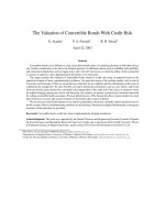
The performance of the binomial model is examined by calculating the-
oretical values of four convertible bonds. The measure used to compare
theoretical values with is the average quote, equal to the average of bid and
ask quotes provided by several financial institutions. We conclude that in
general long historical volatilities and implied volatilities tend to give the
best results. Moreover, we find that our model follows market movements
very well. The impact of different dividend and interest rate scenarios is
rather small.
Keywords: Convertible bonds, hard call, binomial trees
1 Introduction
The global convertible bond markets is very active at the moment, both in
terms of issuance and interest from investors. Convertible bonds are popu-
lar financing vehicles for a diverse range of companies. Possible motives for
a company to issue a convertible bond are, for example, discussed in Bren-
nan (1986)
1
. Figure 1 gives an impression of the development of the global
convertible bond market. The market has grown by 66% in eight years, with
most growth occurring in the USA and Europe.
1990 1992 1994 1996 1998 2000
Year
0
100
200
300
400
Asia
Europe
USA
Japan

Total
Figure 1: Value of the global convertible bond market in $ billion (source:
Deutsche Bank (2001)).
There are different types of convertible bonds. A plain-vanilla convert-
ible bond is a bond that gives the holder the right (but not the obligation)
to exchange a bond for a fixed number of ordinary shares, usually of the
issuer. Usually convertible bonds are redeemed at maturity and they have
fixed coupon payments. The pricing of these bonds is well documented, see
for example Tsiveriotis and Fernandes (1998). In the pricing of such a bond,
the distinction between the debt part and the equity part plays an impor-
tant role. When converting into shares, the right to receive (future) coupon
1
Other references are Barnea, Haugen, and Senbet (1985), Stern (1992), and Lewis, Ragol-
ski, and Seward (1998).
1
payments forgoes. The bond part of a convertible bond is usually described
in terms of Nominal value, Coupon, Number of coupon payments per year,
Issue date and Maturity. The equity part comes up with the Conversion
ratio, which gives the number of underlying shares into which the convert-
ible bond can be converted. The Conversion ratio multiplied by the current
share price is called the Conversion value. By dividing the Nominal value
through the Conversion ratio we find the Conversion price: the price at
which shares are effectively ‘bought’ upon conversion. A convertible bond
is called ‘in the money’ if the share price is higher than the conversion
price.
Market-observed convertible bonds are usually not the plain-vanilla type.
Without being exhaustive, we mention premium redemption, putable, soft
call, callable, step-up, mandatory, parity reset, IPO, multiple currency, per-
petual, exotic, ranking, and reverse convertible bonds. In this paper we will
discuss the pricing of convertible bonds with hard call features. A hard call

feature allows the issuer of a convertible bond to redeem the convertible
bond before maturity by paying a predetermined amount (the call price) to
the investor.
Usually the issuer can exercise the hard call feature after a predeter-
mined date. The period during which the issuer may not redeem a convert-
ible bond under any circumstances is called the hard non-call period. In
addition to the call price the issuer has to pay the accrued interest to the
investor. As soon as the issuer announces to redeem a convertible bond
a notice period starts. During this period (usually approximately 30 days)
bondholders may decide to convert the convertible bond into shares. Of-
ten, the issuer tries to force bondholders to convert into shares in order
to lessen the degree of leverage of the company. Another explanation for
early redemption might be that current financing opportunities are more
attractive than the convertible bond issue.
Convertible bonds are quoted as a percentage of the nominal value. As-
suming a nominal value of
e 1000, we find that the price of a convertible
bond quoted as 91.35% is
e 913.50, excluding accrued interest. Often the
quote is simply 91.35. Call prices are quoted as a percentage of the nominal
value, too.
Sometimes call prices follow a multi-stage scheme. For instance, a con-
vertible bond may be redeemed at 105% during the third year, at 102.5%
during the fourth year and at 100% during the fifth year.
In this paper we discuss a tractable model for the valuation of such con-
vertible bonds with a hard call feature. Prices derived from this model can
be used to value the bonds when they are issued and, perhaps more impor-
tantly, when they are non-traded. The model is a binomial valuation model,
and the value of the bond depends on the characteristics of the underly-
ing stock (especially volatility and dividend payments) and the term struc-

ture. The remainder of this paper is organized as follows. The theoretical
model to value convertible bonds with hard call features is introduced in
section 2. The model is implemented empirically in section 3, and section 4
2
concludes.
2 Modelling Convertible Bonds with Hard Calls Using a
Binomial Tree
Since a convertible bond is a hybrid security that consists of a debt part
and an equity part, it is intuitively logical to value a convertible bond as
the sum of those two components. In this section we develop an option-
like model that can be used to determine the current theoretical value of a
convertible bond with a hard call feature. This value depends of course on
the current values of its underlying debt component and equity component.
The approach adopted here is the binomial tree method developed by Cox,
Ross, and Rubinstein (1979) (the ‘CRR approach’).
The underlying equity of a convertible bond is usually that of the is-
suer. Since the issuer can always deliver his own stock, the equity part is
not exposed to any credit risk. Following Tsiveriotis and Fernandes (1998),
Hull (2000) therefore suggests that the total value of a convertible bond
consists of two components: a risk-free and a risky part. The risk-free part
represents the value of the convertible bond in case it ends as equity, while
the risky part represents the value of the convertible in case it ends as
a bond. Remember, we refer here to credit risk only. Of course, the equity
part is risky because the pay-offs are uncertain, i.e. dependent on future cir-
cumstances. Summing the two components gives the total value of the con-
vertible bond. If we apply the risk-neutral valuation approach, we should
use the risk-free discount rate for the equity part. However, the debt part,
which comprises all payments in cash due to principal and coupon pay-
ments, is subject to risk: cash payments depend on the issuer’s timely ac-
cess to the required cash amounts, and thus introduces credit risk. One

possible way to incorporate credit risk is to reduce the expected payoff of
the debt part. We follow a different approach: we increase the applicable
interest rate. This implies that the debt part should be discounted using
an interest rate that reflects the credit risk of the issuer. The risky inter-
est rate can be determined by adding a credit spread (r
c
) to the risk-free
interest rate (r
f
). This spread is the observable credit spread implied by
non-convertible bonds of the same issuer for maturities similar to the con-
vertible bond. Often the credit spread immediately follows from the credit
rating given to a companies’ debt by rating agencies like Standard & Poor’s
and Moody’s.
The CRR approach is perfectly suited to model convertible bonds with
hard calls. The stock is the underlying value. The life of the binomial tree
should be set equal to the life of the convertible bond. The value of the
convertible bond at the final nodes can be calculated by applying possible
conversion options that the holder has at expiration. Provided that conver-
sion is permitted, the bondholder converts into shares if the conversion
value is greater than the final bond payment (usually the nominal value
plus interest). If the holder does not convert, the final payment is the sum
3
of the nominal value and the final interest payment. Then, by applying the
roll-back procedure, the current value of the convertible bond can be de-
termined. The roll-back procedure has to be applied for both the risk-free
and the risky part. When rolling back through the tree, at each node we
have to determine whether conversion improves the bondholder’s situa-
tion. Suppose that the node under review is node N. When rolling back, the
calculated value of the equity part is equal to

E
N
= e
−r
f
∆t

pE
u
+ (1 − p)E
d

, (1)
while the value of the debt part is equal to
D
N
= e
−(r
f
+r
c
)∆t

pD
u
+ (1 − p)D
d

. (2)
In these expressions, E

u
and D
u
are, respectively, the values of the equity
and the debt part after an up move (relative to node N), while E
d
and D
d
represent the equity and debt values after a down move, and p is the risk-
neutral probability of an upward movement of the stock price. Note that
the credit spread r
c
has entered expression (2). The total roll-back value
R
N
is equal to R
N
= E
N
+ D
N
.
Now suppose that the convertible bond can be converted into shares of
stock. What happens exactly if the bondholder converts? Then the bond-
holder receives CR shares, with conversion value CR ·S
N
, where CR is the
conversion ratio and S
N
represents the share price at node N. If the con-

version value is greater than the roll-back value, it is favorable to convert;
otherwise, the bondholder should not convert. From the discussion above
it follows that the value at node N is equal to
max(CR · S
N
,E
N
+ D
N
). (3)
If conversion takes place, the value of the conversion (CR · S
N
) is risk-free,
so it has to be regarded as the equity part. This means that when the con-
vertible bond is converted, the values of the different components at node
N are:
E
N
= CR ·S
N
,
D
N
= 0,
R
N
= E
N
+ D
N

= CR ·S
N
. (4)
Suppose that a bond is callable at 101% of the nominal value W , where
W = 1000. This means that the issuer can buy back the convertible bond by
paying 1010 to the bondholder. Depending on the share price, the investor
may decide to convert into shares. The issuer’s decision to call a convertible
bond will be a consideration between the call price, the roll-back value (‘do-
nothing value’), and the conversion value.
How can this be formalized and be incorporated in a binomial tree? Let
C
N
be the call price. The issuer tries to minimize the payoff to the investor
and tries to set the value at node N (I
N
)equalto
I
N
= min(R
N
,C
N
). (5)
4
Table 1: Total value at a node under different conditions of a convertible
bond.
Conversion allowed Calling allowed Total value at node
Yes Yes max(min(R
N
,C

N
), CR · S
N
)
Yes No max(R
N
,CR· S
N
)
No Yes min(R
N
,C
N
)
No No R
N
Table 2: Term sheet of imaginary convertible bond XYZ and characteristics
underlying stock XYZ.
Characteristics convertible bond
Nominal value (e) 1000 Conversion ratio 35.7
Coupon 3% Redeems at 100.0%
Frequency 1 Call price 100.5%
Time to maturity (years) 3 Number of steps 3
Risk-free interest rate 5.24% Credit spread 100
(per year, compounded (basis points)
once a year)
Characteristics underlying stock
Stock price (e) 31.25 Volatility (per year) 35%
The bondholder is always allowed to convert if the issuer calls the convert-
ible bond. Therefore, the bondholder will maximize his payoff H

N
:
H
N
= max(I
N
,CR· S
N
). (6)
Substituting expression (5) into (6), we find that the total value at node N
is equal to
max(I
N
,CR· S
N
) = max(min(R
N
,C
N
), CR · S
N
). (7)
Table 1 summarizes the total value at a node for different conversion and
calling possibilities.
The valuation procedure is best understood by using an example. The
characteristics of the convertible bond XYZ and its underlying equity are
given in table 2.
Consequently, the parameters of the binomial tree are as follows:
∆t =
T

n
= 1,
5
u = e
σ
√
∆t
= 1.4191,
d = e
−σ
√
∆t
= 0.7047,
p =
e
r ∆t
− d
u − d
= 0.4867,
d
r
f
=
1
1.0524
= 0.9502,
d
r
=
1

1.0524 + 0.0100
= 0.9413.
T is the time to maturity, ∆t is the length of a time step, r is the risk-free
interest rate , σ is the standard deviation of the return on the share, and u
and d are the ratios by which the share can increase or decrease in value,
respectively. Note that in these formulas the interest rate is transformed
into a continuously compounded interest rate so r is 5.11% . Moreover,
two discount factors are calculated: d
r
f
is used for the risk-free equity
part, while d
r
is used for the risky debt part. Figure 2 shows the bino-
mial tree. At each node four numbers are given: the share price, the equity
part, the debt part and the total value of the convertible bond. At times
t = 1andt = 2 we add the coupon payment (equal to 3) to the debt
component. At the two upper nodes at time t = 3 the convertible bond
is converted into shares, while at the two other nodes the convertible bond
is not converted. At the middle node at time 2 the roll-back value is equal
to R
ud
= 73.22+52.76 = 125.98. The issuer can reduce this value by calling
the convertible bond at 100.50. In addition to the call price the issuer has
to pay the accrued interest, which is equal to 3. Next, the bondholder’s po-
sition can be improved by converting into shares. Therefore, E
ud
becomes
111.56, while D
ud

becomes zero. At the lower node at time t = 1 the roll-
back value is R
d
= 51.60 +51.29 = 102.89. Calling the bond at 103.50 (the
call price plus the accrued interest) does not improve the issuer’s position.
Finally, the current value of the convertible bond is R
0
= 123.16 (at this
node, neither conversion nor calling is allowed). The pure bond value is
B =

3
t=1
3
(1.0624)
t
+
100
(1.0624)
3
= 91.38. This means that the value of the con-
version option (net of the issuer’s call option) is 31.78. Without the hard call
feature the value of the convertible bond would have been 131.23, which
can be calculated in a similar way.
The valuation procedure discussed so far does not take dividend pay-
ments into account. Dividend payments have a non-negligible impact on
share prices, though, so now we incorporate dividend payments in the
valuation tree. The dividend adjustment incorporates known dividends in
the tree. Denote a dividend with ex-dividend date τ (assume τ = i∆t)by
the symbol D

τ
. Straightforward incorporation would result in share prices
S
u
= S
0
u − D
τ
and S
d
= S
0
d − D
τ
at time τ for a specific i. A tree without
dividends has the recombining feature: S
du
= S
ud
. However, in case of a
dividend payment at time τ these two nodes do not recombine. Assuming
that d = 1/u, we find that the share price after a down move from node S
u
6
✑
✑
✑
✑
✑
✑

✑
✑
✑
✑
✑
✑
✑
✑
✑
✑
✑
✑
✑
✑
✑
✑
✑
◗
◗
◗
◗
◗
◗
◗
◗
◗
◗
◗
◗
◗

◗
◗
◗
◗
◗
◗
◗
◗
◗
◗
◗
◗
◗
◗
◗
◗
◗
◗
◗
◗
◗
◗
◗
◗
◗
◗
◗
◗
◗
◗

◗
◗
◗
✑
✑
✑
✑
✑
✑
✑
✑
✑
✑
✑
✑
✑
✑
✑
✑
✑
✑
✑
✑
✑
✑
✑
312.50 (Share price)
983.80 (Equity part)
247.80 (Debt part)
1231.60 (Convertible

bond)
443.50
1583.20
0
1583.20
220.20
516.00
512.90
1028.90
629.30
2246.60
0
2246.60
312.50
1115.60
0
1115.60
155.20
0
999.50
999.50
893.00
3188.10
0
3188.10
443.50
1583.20
0
1583.20
220.20

0
1030.00
1030.00
109.40
0
1030.00
1030.00
t = 0 t = 1 t = 2 t = 3
Figure 2: Binomial tree for convertible bond.
7
becomes S
ud
= (S
0
u − D
τ
)d, while the share price after an up move from
node S
d
becomes S
du
= (S
0
d −D
τ
)u.SinceS
ud
≠ S
du
, the tree does not re-

combine. This direct approach to modelling dividend payments creates too
many nodes: the number of nodes grows exponentially with the number of
time periods until maturity. In order to reduce calculation time, the model
should deal with dividend payments in a more efficient way.
Hull (2000) discusses a modification that overcomes this problem. The
basic idea is to split the share price into two components: a certain part and
an uncertain part that is the present value of all future dividends during the
lifetime of the convertible bond. Define S
u
and σ
u
as the uncertain part of
the stock and its volatility, respectively. Assume that 0 <τ<T, where
T represents the expiration of the convertible bond. Then, at time i∆t we
have:
S
u
=

S − D
τ
e
−r
f
(τ−i∆t)
∀i∆t ≤ τ
S ∀i∆t>τ
(8)
After substituting σ
u

in the expressions for u, d,andp, the tree can be
calculated, following the normal roll-back procedure. Next, we have to add
the present value of the dividend payment. The share price at time t = i∆t
is given by the following expression:
S =

S
u
0
u
j
d
i−j
+ D
τ
e
−r
f
(τ−i∆t)
j = 0, 1, i,∀i∆t ≤ τ
S
u
0
u
j
d
i−j
j = 0, 1, i,∀i∆t>τ
(9)
This procedure can easily be extended to a stock paying more than one

dividend.
Until now, we have assumed that the term structure of interest rates is
flat. In reality, of course, this is not the case so we need to extend the valu-
ation procedure to take the entire zero-coupon yield curve into account.
Assume that the zero-coupon curve consists of n points. Let the sym-
bols t
i
and R
i
denote the maturity and the continuously compounded yield,
on a yearly basis, of point i on the zero-coupon curve (1 ≤ i ≤ n). The con-
cordant short-term interest rates in each time interval are derived from the
expectations theory (see for example Cochrane (2001) for a recent exposi-
tion). The expectations theory states that long-term interest rates should
reflect expected future short-term interest rates: the forward interest rate
for a certain future period should be equal to the expected future zero-
coupon rate for that period.
Let F
i
denote the forward rate between time t
i−1
and t
i
. To calculate the
forward rate F
i
, the following equation must hold:
e
t
i−1

R
i−1
e
(t
i
−t
i−1
)F
i
= e
t
i
R
i
. (10)
Solving for F
i
gives
F
i
=
t
i
R
i
− t
i−1
R
i−1
t

i
− t
i−1
. (11)
8
Situation 2
Situation 1
t
i
t
i+1
t
i+2
j∆t(j+ 1)∆t
t
i
t
i+1
j∆t(j+ 1)∆t
Figure 3: Two different situations that may arise when using forward rates
in a binomial tree.
Expression (11) is used to calculate the forward rates between the nodes of
a tree. Several situations may occur. In figure 3, two different situations are
drawn.
In general the time intervals ∆t are rather small. For this reason, situa-
tion 1 is most likely to occur. In this case, the forward interest rate between
node j and node j + 1isequaltoF
i+1
=
t

i+1
R
i+1
−t
i
R
i
t
i+1
−t
i
. This means that the
risk-neutral probability of an up move between node j and node j +1isas
follows:
p =
e
F
i+1
∆t
− d
u − d
(12)
The second possibility is slightly more complicated. In that case, the matu-
rity of a zero-coupon yield falls between two nodes, so that during this time
interval we have two different zero-coupon yields. The forward interest rate
in this interval is
F

=


(j + 1)∆t − t
i+1

F
i+2
+

t
i+1
− j∆t

F
i+1
∆t
. (13)
Forward rate F

should be used to calculate the probability p in equa-
tion (12). Obviously, the two situations given above do not cover all possibil-
ities. For instance, another point of the zero-coupon curve can fall between
two nodes. In this case, the forward rate should be calculated analogously
to the calculation of F

.
Summarizing, we model the value of a convertible bond with a hard call
feature by the following steps:
9
10 20 30 40 50
Stock
80

100
120
140
160
180
Bond
Conversion value
Convertible with hard call
Convertible without hard call
Figure 4: Value of convertible bond with and without hard call feature, con-
version value and pure bond value versus share price.
• a CRR binomial tree was used to calculate the value of a convertible
bond, thereby distinguishing between a risk-free and a risky compo-
nent;
• the binomial tree was modified to include issuer’s hard call features;
• dividends to be paid out during the lifetime of the convertible bond
were incorporated;
• the model was adjusted to take the entire zero-coupon yield curve
into account.
In the remainder of this section we show how the value of the bond de-
pends on its characteristics. The characteristics of the convertible bond are
specified in table 2.
In figure 4, the value of a convertible bond (with and without hard call
feature) and the conversion value are drawn versus the share price. Also,
the pure bond value is displayed. A convertible bond without a hard call
feature has a higher value than a convertible bond with a hard call fea-
tures: the hard call feature is unfavorable for the bondholder and therefore
reduces the value of the convertible bond.
10
0 1020304050

Value of stock
0.0
0.2
0.4
0.6
0.8
1.0
delta bond with hard-call feature
delta bond without hard-call feature
Figure 5: Delta of convertible bond versus share price.
Figure 4 also shows that for relatively low share prices (compared to
the conversion price) the values of the convertible bond with and without
hard call are equal to the pure bond value. For low share prices the convert-
ible bond behaves like a bond, while for high share prices the convertible
bond behaves like the underlying equity (in this case, 35.7 shares). This
can be concluded from the following figure, too: in figure 5 the delta of
the convertible bond is drawn. (Delta is the rate of change of the price of
a derivative with the price of the underlying equity, 35.7 shares in our ex-
ample, so delta equals
∂CB
∂(35.7S)
.) For low share prices the delta is almost 0,
while for high share prices the delta converges to 1.
Figure 6 shows the effect of an increase of the volatility of the under-
lying share price. A higher volatility increases the probability that a high
share price will be reached, so that the value of the convertible bond in-
creases. This can be understood as well by seeing the convertible bond in
terms of an option and a pure bond, thereby neglecting the issuer’s call. A
higher volatility increases the value of the option and leaves the value of
the bond unchanged, so that the value of the convertible bond increases. In

figure 7 we show the impact of a longer time to maturity. Since the risky in-
terest rate (6.24%) is higher than the coupon (3%), a longer time to maturity
reduces the pure bond value. However, a longer time to maturity increases
11
10 15 20 25 30 35 40
Value of stock
80
100
120
140
160
Volatility 25%
Volatility 35%
Volatility 45%
Figure 6: Value convertible bond with hard call for different volatilities ver-
sus share price.
12
10 15 20 25 30 35 40
Value of stock
80
100
120
140
160
Time to maturity: three years
Time to maturity: four years
Time to maturity: five years
Figure 7: Value convertible bond with hard call for different times to matu-
rity versus share price.
the value of the implied option. Figure 7 illustrates the net impact of these

opposite effects. For low share prices, the debt part dominates the equity
part, so the reduction of the pure bond value exceeds the increase of the
value of the implied option. For high share prices the net impact of a longer
time to maturity is the reverse: the value of the convertible bond increases.
In the next section we put our valuation model to test: we will calculate
theoretical values of four convertible bonds. These theoretical values will
be compared to market-observed prices.
3 Empirical Results of the Binomial Valuation Model
In this section we use the valuation model of the previous section to calcu-
late theoretical prices of three convertible bonds. Two remarks have to be
made. First, in reality the time at which zero coupon rates and concordant
forward rates are applicable, does not always coincide with the chosen time
step at the binomial tree. Second, the timing of the observed payments does
not always coincide with the points in time of the tree.
The bonds we consider are Ahold 3% 1998-2003, Ahold 4% 2000-2005,
13
and ASML 2.5% 1998-2005; details on these specific bonds can be found
in Appendix A. We will compare these theoretical prices with those that
were observed in practice, and we examine how sensitive the results of the
model are to some of the parameters that need to be estimated.
The convertible bond market is not very liquid, and consequently mar-
ket prices can be outdated. For this reason we compare the theoretical val-
ues with quotes given by financial institutions. These quotes are indicative
prices against which banks are prepared to trade convertible bonds. Invest-
ment banks like ABN AMRO, UBS Warburg, and Morgan Stanley Dean Witter
provide quotes on a real time basis. The measure used to compare theoret-
ical values with is the average quote (Q). The average quote is the average
of all bid and ask quotes provided by these banks:
Q =
1

2N



i
B
i
+

i
A
i


. (14)
In this expression, B
i
and A
i
represent the bid and the ask quote of bank i,
respectively, while N represents the total number of quotes used. Quotes
not updated regularly were left out. Moreover, we omitted bad quotes. An
example of a bad quote is one that is below the pure bond value. Most
times, at least fourteen banks provide useful quotes. The data used for the
empirical analysis consist of more than 1600 observations. During three
weeks (23 October to 17 November 2000 ), every five minutes we stored
all relevant parameters: the price of the underlying stock, risk-free interest
rates, all quotes, etc.
Most of the parameters of the valuation model (for instance the time
to maturity) are known with certainty. However, some parameters cannot

be determined unambiguously and thus have to be estimated. The param-
eters to be estimated are the volatility, the dividends to be paid out during
the lifetime of the convertible bond, and the risk-free interest rate. In the
next three subsections, we will carry out a valuation analysis including a
sensitivity analysis with respect to these three parameters.
3.1 Volatility Analysis
First, we consider estimation of the volatility. The volatility can be deter-
mined by either using historical data or by calculating the implied volatility
from current option prices.
To estimate the volatility of a stock empirically from historical stock
prices, the stock price has to be observed at fixed intervals of time. In this
volatility analysis, we calculated the historical volatility based on closing
prices of the last 5, 10, 20, 30, 50, and 100 trading days
2
. Let the continu-
ously compounded return u
i
on day i be calculated as ln(S
i
+δ
i
D
i
)−ln S
i−1
,
2
Alternatively, we could estimate the volatility using a (G)ARCH-model, but we do not
pursue that direction here.
14

with δ
i
an indicator which is 1 if day i is a dividend day. The n-day volatility
is now calculated as
σ
n
=
1
TD




1
n − 1

i
(
u
i
−
¯
u
)
2
with TD the length of a time interval in a year. TD can be measured in
calendar days or in trading days. Fama (1965) and French (1980) show that
volatility is far larger when the exchange is open than when it is closed.
French and Roll (1986) conclude that volatility is largely caused by trading
itself. These results suggest that we should measure TD in trading days.

Since the average number of trading days over the last five years was 253,
we use TD = 1/253.
Implied volatilities are derived from call options, with preferably the
same time to maturity as the convertible bond. However, these series may
not be very liquid, so we also consider option series with a shorter time to
maturity. We distinguish between volatility implied by a short running op-
tion series (this series matures in October 2001), and the volatility implied
by series maturing either in October 2003 (in the case of the Ahold 3% con-
vertible) and October 2005 (in the case of the Ahold 4% convertible). For the
analysis of the ASML 2.5% convertible, we used option series running until
October 2001 and October 2005. We will refer to these volatility estimates
as short and long implied volatility estimates.
Finally, dividend predictions were obtained from the merchant bank
Kempen&Co
3
, and we used two yield curves: a single yield curve and the
actual zero-coupon yield curve (see also subsection 3.3).
Because of the high frequency nature of the data, we select two observa-
tions for each day, one at 12.00 am and one at 4.00 pm. This leaves us with
36 observations per case. The interpretation of the results is made easier
by selecting these observations, since the original observations (taken at
5-minutes intervals) are strongly dependent, and the selected observations
display much weaker dependence over time. Unless indicated otherwise, we
use this set of 36 observations to assess the fit of the theoretical values to
the observed prices.
In Figures 8-9, we graph the average prices of the convertible bonds
and the theoretical values. Average.mid is the average of the bid and ask
quotes (equation 14). Two choices for the volatility estimate are shown in
the graphs: zc.100 is based on historical volatility of the last 100 trading
days, and zc.ivl is based on the volatility implied by the option series with

duration until maturity of the bond. In both cases, the risk free interest is
derived from the zero-coupon interest structure.
In Table 3, we list the correlation between the theoretical value and the
average quote for all estimates of the volatility (all correlations are calcu-
lated using the 36 selected observations). The distribution of the relative
3
This bank is now part of Dexia Securities.
15
50 300 550 800 1050 1300 1550 1800
118
120
122
124
126
128
130
Average.mid
zc.100
zc.ivl
50 300 550 800 1050 1300 1550 1800
110
112
114
116
118
120
Average.mid
zc.100
zc.ivl
Figure 8: Theoretical values and average quote Ahold 3% (top) and Ahold

4% (bottom) (zero-coupon interest structure).
16
50 300 550 800 1050 1300 1550 1800
130
140
150
160
170
180
Average.mid
zc.100
zc.ivl
Figure 9: Theoretical values and average quote ASML (zero-coupon interest
structure).
17
AHOLD 3% AHOLD 4% ASML
ZC SY ZC SY ZC SY
Hist. 5 0.981 0.981 0.836 0.825 0.916 0.917
Hist. 10 0.987 0.987 0.961 0.957 0.949 0.950
Hist. 20 0.983 0.983 0.948 0.940 0.991 0.991
Hist. 30 0.980 0.944 0.941 0.946 0.991 0.991
Hist. 50 0.944 0.980 0.446 0.453 0.994 0.994
Hist. 100 0.972 0.972 0.954 0.953 0.993 0.993
IV short 0.981 0.981 0.871 0.873 0.947 0.985
IV long 0.983 0.983 0.929 0.932 0.993 0.993
Table 3: Correlation between average quotes and theoretical values for sev-
eral choices of volatility.
errors are shown in the box-and-whisker plots in Figure 10
4
.

We see from Table 3 and Figures 8-9 that the model tracks the observed
average prices reasonably well. The correlation between the theoretical val-
ues and observed prices exceeds, for almost all choices of volatility, 0.90.
There is no single volatility measure that gives the best estimate for the
average quote. However, in general the long historical and implied volatil-
ities give reasonably good results. This is shown in Figure 10, where er-
ror distributions corresponding to these choices of volatility estimates are
more concentrated around zero. For the Ahold 3% and Ahold 4% convert-
ible bonds, the average quotes tend to be underestimated by the model, for
the ASML convertible bond the average quote is overestimated. In the case
of the Ahold 3% convertible, this bias appears for all cases, that is, for all
measures of volatility and for both the single yield and zero-coupon inter-
est structure. In the case of the Ahold 4% convertible, the observed price of
the bond is higher than the value resulting from the model for all choices
of volatility estimate except the one based on the long implied volatility. In
that case, the actual price is lower than the one from the binomial valuation
model. From Table 3 we see that the correlation between the model value
and the observed value is very low in case of the historic 50-day volatility
(compared to the price correlations resulting from other choices of volatil-
ity estimates). This can be explained by the sharp rise of the price of the
underlying share in the end of October. The price of the stock stabilized
again early November. This caused a significant drop of the 50-day histor-
ical volatility. Historical volatilities based on less than 50 days adjusted
more quickly than the other volatilities.
From Table 3 and Figure 10 we see that the correlation between the
theoretical value and the average quote is also very high for the ASML 2.5%
convertible bond. The distribution of the relative errors is more dispersed
than those of the AHOLD convertibles. The average quote is overestimated
on average, but the relative error is small if the volatility estimate is based
4

In these box-and-whisker plots, the lower side box indicates the first quartile, and the
upper side the third quartile of the distribution of relative errors. The horizontal line in each
box is the median. The whiskers indicate the minimum and maximum relative error.
18
-0.10 -0.05 0.0 0.05 0.10
H5 H10 H20 H30 H50 H100 ivs ivl
Rel. error Ahold 3% SY
-0.10 -0.05 0.0 0.05 0.10
H5 H10 H20 H30 H50 H100 ivs ivl
Rel. error Ahold 3% ZC
-0.10 -0.05 0.0 0.05 0.10
H5 H10 H20 H30 H50 H100 ivs ivl
Rel. error Ahold 4% SY
-0.10 -0.05 0.0 0.05 0.10
H5 H10 H20 H30 H50 H100 ivs ivl
Rel. error Ahold 4% ZC
-0.10 -0.05 0.0 0.05 0.10
H5 H10 H20 H30 H50 H100 ivs ivl
Rel. error ASML 2.5% SY
-0.10 -0.05 0.0 0.05 0.10
H5 H10 H20 H30 H50 H100 ivs ivl
Rel. error ASML 2.5% ZC
Figure 10: Boxplots of relative error of theoretical valuation.
19
on long historical data or the long implied volatility.
We conclude this subsection by summarizing our main findings. The bi-
nomial valuation model is reasonably well able to model the average quotes.
There is no single volatility measure that estimates the average quote best,
but in general long historical and implied volatilities give better results.
3.2 Dividend Analysis

In this subsection we examine how sensitive the valuations by the binomial
valuation model are to different estimates of the dividends to be paid out
during the lifetime of the convertible bond. Since ASML does not pay any
dividends, we consider the two Ahold convertible bonds only.
The basic estimates of future dividends are provided by Kempen & Co
Research. We have used these estimates in the previous subsection. To es-
timate impact of different dividend estimates on theoretical prices, we cal-
culate four other scenarios in which the dividends are 80%, 90%, 110% and
120% of the Kempen & Co Research estimates. The volatility used in the
analysis is the long implied volatility, which provided a reasonable fit as
seen in the previous subsection. Somewhat arbitrarily, we consider four
different dividend scenarios, in which the dividends are 80%, 90%, 110%
and 120% of the baseline estimates.
Higher dividend payments reduce the value of the convertible bond.
The reductions of the values of the convertible bonds due to an increase of
the dividend payments are seen both for the Ahold 3% convertible and the
Ahold 4% convertible, and do not depend on the interest structure chosen.
The Ahold 4% convertible bond is most sensitive to changes of the dividend
estimates: on average, the bond loses 0.5% in value when dividends increase
by 10%. The same quantity is only 0.2% for the Ahold 3% convertible. This
is due to the longer time to maturity (2005 versus 2003) of the Ahold 4%
convertible.
3.3 Interest Rate Analysis
The last parameter in the binomial valuation model that needs to be chosen
is the risk-free interest rate. Previously, little attention was paid to the risk-
free interest rates used to calculate theoretical values and in this section we
are more precise. We distinguished between two different term structures
of interest rates: a full zero-coupon term structure (ZC) and a single-yield
term structure (SY). The single yield is the yield to maturity on Dutch gov-
ernment bonds. The expiration of this government bond is the expiration

that matches best with the expiration of the convertible bond. The single
yields are, for example, given by Reuters on a real time basis. The zero-
coupon term structure can be found on Reuters as well and is derived from
swap rates.
We use the zero-coupon curve based on the euro. To examine the im-
pact of a different term structure, for both structures the interest rates are
lowered and increased by 10 and 25 basis points (±0.10%, ±0.25%). The
20
volatility used is the long implied volatility. In Figure 11 we display the
relative error of the valuation under different terms structures of interest
rates.
If we look at the valuations at different times, it turns out that an up-
ward shift of the yield curve reduces the theoretical value of a convert-
ible bond. Especially the Ahold 4% convertible bond is quite sensitive with
respect to interest rate changes, which is explained by the long time to
maturity. However, we do not observe this for the ASML convertible bond,
which has more or less the same time to maturity. Since this convertible
bond is far in-the-money, the equity part dominates the debt part. Conse-
quently, the convertible bond behaves like equity and is, keeping all other
factors constant, not very sensitive to interest rate changes. The relative
error distributions in Figure 11 do not vary much by the yield curve that
is chosen. Therefore, a shift of the yield curve does not change theoretical
values enormously, especially if the convertible bond is in-the-money. For
example, on October 23 2000, 16.00hrs, the model value of the Ahold 4%
convertible with zero-coupon rates was 114.98, and with single yield rates
115.80 (both numbers are calculated using the long implied volatility es-
timate). Shifting the yield curve upwards by 25 basis points decreases the
zero coupon valuation to 114.52, shifting it downwards by 25 basis points
changes the zero coupon valuation to 115.33.
4 Conclusions and Directions for Further Research

In this paper we have proposed a binomial valuation model for convert-
ible bonds with hard call features. The model distinguishes between a debt
component and an equity component of the bond. It takes dividend pay-
ments during the life time of the bond into account, as well as the actual
yield curve.
In section 3 we compared the theoretical valuations with the market
prices of three different convertible bonds. In general, the binomial valu-
ation model tracks the actual quotes quite well. The correlation between
the theoretical value and the actual average quotes exceeds 0.95 for almost
all choices of volatility estimates, dividend policy, and term structure of
interest rates.
We examined in detail how sensitive the valuations are to the three pa-
rameters. It was found that the results are sensitive to the estimate of the
volatility of the underlying stock, and much less so to the estimate of divi-
dend payout and the choice of the specific term structure of interest rates.
Of course, this depends on the level of the underlying stock price. Estimates
of volatility based on long historic data of the stock, or on the volatility im-
plied by call-options with a long life time tend to give the best results.
In future research we will use a similar approach to the valuation of
convertible bonds with soft call features. These bonds are convertible only
if the level of the stock price has exceeded a prescribed level for a certain
amount of time. This creates state dependence in the binomial tree, and
21
-0.04 -0.02 0.0 0.02 0.04
M25 M10 P10 P25
Rel. error Ahold 3% SY
-0.04 -0.02 0.0 0.02 0.04
M25 M10 P10 P25
Rel. error Ahold 3% ZC
-0.04 -0.02 0.0 0.02 0.04

M25 M10 P10 P25
Rel. error Ahold 4% SY
-0.04 -0.02 0.0 0.02 0.04
M25 M10 P10 P25
Rel. error Ahold 4% ZC
-0.04 -0.02 0.0 0.02 0.04
M25 M10 P10 P25
Rel. error ASML 2.5% SY
-0.04 -0.02 0.0 0.02 0.04
M25 M10 P10 P25
Rel. error ASML 2.5% ZC
Figure 11: Boxplots of relative error of theoretical valuation.
22
therefore valuation using methodology based on partial differential equa-
tion seems to hold more promise.
References
Barnea, A., R.A. Haugen, and L.W. Senbet (1985). Agency Problems and
Financial Contracting. Englewood Cliffs: Prentice Hall.
Brennan, M. (1986). The case for convertibles. In J.M. Stern and D.H. Chew
(Eds.), The Revolution in Corporate Finance, New York, pp. 163–171.
Basil Blackwell.
Cochrane, J.H. (2001). Asset Pricing. Princeton: Princeton University Press.
Cox, J.C., S.A. Ross, and M. Rubinstein (1979). Option pricing: A simplified
approach. Journal of Financial Economics 7, 229–263.
Deutsche Bank (2001). www.dbconvertibles.com. (website).
Fama, E.E. (1965). The behavior of stock market prices. Journal of Busi-
ness 38, 35–105.
French, K.R. (1980). Stock returns and the weekend effect. Journal of Fi-
nancial Economics 8, 55–69.
French, K.R. and R. Roll (1986). Stock return variances: The arrival of in-

formation and the reaction of traders. Journal of Financial Economics
17, 5–26.
Hull, J.C. (2000). Options, Futures & Other Derivatives (fourth ed.). Lon-
don: Prentice-Hall.
Lewis, C.M., R.J. Ragolski, and J.K. Seward (1998). Understanding the de-
sign of convertible debt. The Journal of Applied Corporate Finance 11,
45–53.
Stern, J.M. (1992). Convertible bopnds as backdoor equity financing. Jour-
nal of Financial Economics 32, 3–21.
Tsiveriotis, K. and C. Fernandes (1998). Valuing convertible bonds with
credit risk. The Journal of Fixed Income 8, 95–102.
23