Small functional equations and how to solve them (PBM)
Bạn đang xem bản rút gọn của tài liệu. Xem và tải ngay bản đầy đủ của tài liệu tại đây (823.06 KB, 138 trang )
Problem Books in Mathematics
Edited by P. Winkler
Problem Books in Mathematics
Series Editor: Peter Winkler
Pell’s Equation
by Edward J. Barbeau
Polynomials
by Edward J. Barbeau
Problems in Geometry
by Marcel Berger, Pierre Pansu, Jean-Pic Berry, and Xavier Saint-Raymond
Problem Book for First Year Calculus
by George W. Bluman
Exercises in Probability
by T. Cacoullos
Probability Through Problems
by Marek Capin´ski and Tomasz Zastawniak
An Introduction to Hilbert Space and Quantum Logic
by David W. Cohen
Unsolved Problems in Geometry
by Hallard T. Croft, Kenneth J. Falconer, and Richard K. Guy
Berkeley Problems in Mathematics, (Third Edition)
by Paulo Ney de Souza and Jorge-Nuno Silva
The IMO Compendium: A Collection of Problems Suggested for the
International Mathematical Olympiads: 1959-2004
by Dusˇan Djukic´, Vladimir Z. Jankovic´, Ivan Matic´, and Nikola Petrovic´
Problem-Solving Strategies
by Arthur Engel
Problems in Analysis
by Bernard R. Gelbaum
Problems in Real and Complex Analysis
by Bernard R. Gelbaum
(continued after index)
Christopher G. Small
Functional Equations
and How to Solve Them
Mathematics Subject Classification (2000): 39-xx
Library of Congress Control Number: 2006929872
ISBN-10: 0-387-34534-5 e-ISBN-10: 0-387-48901-0
ISBN-13: 978-0-387-34534-5 e-ISBN-13: 978-0-387-48901-8
Printed on acid-free paper.
© 2007 Springer Science+Business Media, LLC
All rights reserved. This work may not be translated or copied in whole or in part without the
written permission of the publisher (Springer Science+Business Media, LLC, 233 Spring Street,
New York, NY 10013, USA), except for with reviews or scholarly analysis. Use in connection
with any form of information storage and retrie computer software, or by similar or dissimilar
methodology now known or hereafter developed is forbidden.
The use in this publication of trade names, trademarks, service marks, and similar terms, even if
they are not identified as such, is not to be taken as an expression of opinion as to whether or
not they are subject to proprietary rights.
987654321
springer.com
Christopher G. Small
Department of Statistics & Actuarial Science
University of Waterloo
200 University Avenue West
Waterloo N2L 3G1
Canada
Series Editor:
Peter Winkler
Department of Mathematics
Dartmouth College
Hanover, NH 03755
USA
2
x
1-1
f(x)
-1
-1.5
0-2
1.5
0
1
0.5
2
-0.5
f(x)+f(2 x)+f(3 x)=0
for all real x.
This functional equation is satisfied by the function f(x) ≡ 0, and also by
the strange example graphed above. To find out more about this function, see
Chapter 3.
2
x
0
-2
4
-4
20-2-4
f(x)
4
f(f(f(x))) = x
Can you discover a function f(x) which satisfies this functional equation?
Contents
Preface ix
1 An historical introduction 1
1.1 Preliminaryremarks 1
1.2 NicoleOresme 1
1.3 GregoryofSaint-Vincent 4
1.4 Augustin-LouisCauchy 6
1.5 Whataboutcalculus? 8
1.6 Jeand’Alembert 9
1.7 CharlesBabbage 10
1.8 Mathematicscompetitionsandrecreationalmathematics 16
1.9 Acontribution fromRamanujan 21
1.10 Simultaneous functional equations 24
1.11 Aclarificationofterminology 25
1.12 Existenceand uniquenessofsolutions 26
1.13 Problems 26
2 Functional equations with two variables 31
2.1 Cauchy’sequation 31
2.2 ApplicationsofCauchy’sequation 35
2.3 Jensen’sequation 37
2.4 Linear functional equation 38
2.5 Cauchy’sexponential equation 38
2.6 Pexider’sequation 39
2.7 Vincze’s equation 40
2.8 Cauchy’sinequality 42
2.9 Equations involving functions of two variables 43
2.10 Euler’sequation 44
2.11 D’Alembert’sequation 45
2.12 Problems 49
viii Contents
3 Functional equations with one variable 55
3.1 Introduction 55
3.2 Linearization 55
3.3 Some basic families of equations 57
3.4 Amenagerieofconjugacyequations 62
3.5 Findingsolutionsfor conjugacyequations 64
3.5.1 The Koenigs algorithm for Schr¨oder’sequation 64
3.5.2 The L´evyalgorithmfor Abel’sequation 66
3.5.3 An algorithm for B¨ottcher’s equation 66
3.5.4 Solving commutativity equations 67
3.6 Generalizations of Abel’s and Schr¨oder’sequations 67
3.7 Generalpropertiesofiterativeroots 69
3.8 Functional equationsand nestedradicals 72
3.9 Problems 75
4 Miscellaneous methods for functional equations 79
4.1 Polynomialequations 79
4.2 Powerseriesmethods 81
4.3 Equations involving arithmetic functions 82
4.4 Anequationusing specialgroups 87
4.5 Problems 89
5 Some closing heuristics 91
6 Appendix: Hamel bases 93
7 Hints and partial solutions to problems 97
7.1 Awarningtothereader 97
7.2 Hintsfor Chapter1 97
7.3 Hintsfor Chapter2 102
7.4 Hintsfor Chapter3 107
7.5 Hintsfor Chapter4 113
8 Bibliography 123
Index 125
Preface
Over the years, a number of books have been written on the theory of func-
tional equations. However, few books have been published on solving func-
tional equations which arise in mathematics competitions and mathematical
problem solving. The intention of this book is to go some distance towards
filling this gap.
This work began life some years ago as a set of training notes for
mathematics competitions such as the William Lowell Putnam Competition
for undergraduate university students, and the International Mathematical
Olympiad for high school students. As part of the training for these competi-
tions, I tried to put together some systematic material on functional equations,
which have formed a part of the International Mathematical Olympiad and a
small component of the Putnam Competition. As I became more involved
in coaching students for the Putnam and the International Mathematical
Olympiad, I started to understand why there is not much training mate-
rial available in systematic form. Many would argue that there is no theory
attached to functional equations that are encountered in mathematics compe-
titions. Each such equation requires different techniques to solve it. Functional
equations are often the most difficult problems to be found on mathematics
competitions because they require a minimal amount of background theory
and a maximal amount of ingenuity. The great advantage of a problem involv-
ing functional equations is that you can construct problems that students at
all levels can understand and play with. The great disadvantage is that, for
many problems, few students can make much progress in finding solutions even
if the required techniques are essentially elementary in nature. It is perhaps
this view of functional equations which explains why most problem-solving
texts have little systematic material on the subject. Problem books in mathe-
matics usually include some functional equations in their chapters on algebra.
But by including functional equations among the problems on polynomials or
inequalities the essential character of the methodology is often lost.
As my training notes grew, so grew my conviction that we often do not do
full justice to the role of theory in the solution of functional equations. The
x Preface
result of my growing awareness of the interplay between theory and problem
application is the book you have before you. It is based upon my belief that
a firm understanding of the theory is useful in practical problem solving with
such equations. At times in this book, the marriage of theory and practice is
not seamless as there are theoretical ideas whose practical utility is limited.
However, they are an essential part of the subject that could not be omit-
ted. Moreover, today’s theoretical idea may be the inspiration for tomorrow’s
competition problem as the best problems often arise from pure research. We
shall have to wait and see.
The student who encounters a functional equation on a mathematics con-
test will need to investigate solutions to the equation by finding all solutions
(if any) or by showing that all solutions have a particular property. Our em-
phasis is on the development of those tools which are most useful in giving a
family of solutions to each functional equation in explicit form.
At the end of each chapter, readers will find a list of problems associated
with the material in that chapter. The problems vary greatly in difficulty,
with the easiest problems being accessible to any high school student who has
read the chapter carefully. It is my hope that the most difficult problems are
a reasonable challenge to advanced students studying for the International
Mathematical Olympiad at the high school level or the William Lowell Put-
nam Competition for university undergraduates. I have placed stars next to
those problems which I consider to be the harder ones. However, I recognise
that determining the level of difficulty of a problem is somewhat subjective.
What one person finds difficult, another may find easy.
In writing these training notes, I have had to make a choice as to the gen-
erality of the topics covered. The modern theory of functional equations can
occur in a very abstract setting that is quite inappropriate for the readership
I have in mind. However, the abstraction of some parts of the modern theory
reflects the fact that functional equations can occur in diverse settings: func-
tions on the natural numbers, the integers, the reals, or the complex numbers
can all be studied within the subject area of functional equations. Most of the
time, the functions I have in mind are real-valued functions of a single real
variable. However, I have tried not to be too restrictive in this. The reader will
also find functions with complex arguments and functions defined on natural
numbers in these pages. In some cases, equations for functions between circles
will also crop up. Nor are functional inequalities ignored.
One word of warning is in order. You cannot study functional equations
without making some use of the properties of limits and continuous functions.
The fact is that many problems involving functional equations depend upon
an assumption of such as continuity or some other regularity assumption that
would usually not be encountered until university. This presents a difficulty
for high school mathematics contests where the properties of limits and conti-
nuity cannot be assumed. One way to get around this problem is to substitute
another regularity condition that is more acceptable for high school mathe-
matics. Thus a problem where a continuity condition is natural may well get
Preface xi
by with the assumption of monotonicity. Although continuity and monotonic-
ity are logically independent properties (in the sense that neither implies the
other) the imposition of a monotonicity condition in a functional equations
problem may serve the same purpose as continuity. Another way around the
problem is to ask students to provide a weaker conclusion that is not “finished”
by invoking continuity. Asking students to determine the nature of a function
on the rational numbers is an example of this. Neither solution to this problem
is completely satisfactory. Fortunately, there are enough problems which can
be posed and solved using high school mathematics to serve the purpose. More
advanced contests such as the William Lowell Putnam Competition have no
such restrictions in imposing continuity or convexity, and expect the student
to treat these assumptions with mathematical maturity.
Some readers may be surprised to find that the chapter on functional
equations in a single variable follows that on functional equations in two or
more variables. However this is the correct order. An equation in two or more
variables is formally equivalent to a family of simultaneous equations in one
variable. So equations in two variables give you more to play with. I have
had to be very selective in choosing topics in the third chapter, because much
of the academic literature is devoted to establishing uniqueness theorems for
solutions within particular families of functions: functions that are convex or
real analytic, functions which obey certain order conditions, and so on. It
would be easy to simply ignore the entire subject if it were not for the fact
that functional equations in a single variable are commonplace in mathematics
competitions. So I have done my best to present those tools and unifying
concepts which occur periodically in such problems in both high school and
university competitions. Chapter 3 has been written with a confidence that
advanced high school students will adapt well to the challenge of a bit of
introductory university level mathematics. The chapters can be read more-or-
less independently of each other. There are some results in later chapters which
depend upon earlier chapters. However, the reader who wishes to sample the
book in random order can probably piece together the necessary information.
The fact that it is possible to write a book whose chapters are not heavily
dependent is a consequence of the character of functional equations. Unlike
some branches of mathematics, the subject is wide, providing easier access
from a number of perspectives. This makes it an excellent area for competition
problems. Even tough functional equations are relatively easy to state and
provide lots of “play value” for students who may not be able to solve them
completely.
Because this is a book about problem solving, the reader may be surprised
to find that it begins with a chapter of the history of the subject. It is my
belief that the present way of teaching mathematics to students puts much
emphasis on the tools of mathematics, and not enough on the intellectual
climate which gave rise to these ideas. Functional equations were posed and
solved for reasons that had much to do with the intellectual challenges of
xii Preface
their times. This book attempts to provide a small glimpse of some of those
reasons.
I have learned much about functional equations from other people. This
book also owes much to others. So this preface would not be complete with-
out some mention of the debts that I owe. I have learned much from the
work of Janos Acz´el, Distinguished Professor Emeritus at the University of
Waterloo. The impact of his work and that of his colleagues is to be found
throughout the following pages in places too numerous to mention. The initial
stages of this monograph were written at the instigation of Pat Stewart and
Richard Nowakowski. Sadly, Pat Stewart is no longer with us, and is missed
by the mathematical community. Thank you, Patrick and Richard. Finally, I
would like to thank Professor Ed Barbeau, who generously sent some of his
correspondence problems to me. His encouragement and assistance are much
appreciated.
1
An historical introduction
1.1 Preliminary remarks
In high school algebra, we learn about algebraic equations involving one or
more unknown real numbers. Functional equations are much like algebraic
equations, except that the unknown quantities are functions rather than real
numbers. This book is about functional equations: their role in contempo-
rary mathematics as well as the body of techniques that is available for their
solution. Functional equations appear quite regularly on mathematics com-
petitions. So this book is intended as a toolkit of methods for students who
wish to tackle competition problems involving functional equations at the high
school or university level.
In this chapter, we take a rather broad look at functional equations. Rather
than focusing on the solutions to such equations—a topic for later chapters—
we show how functional equations arise in mathematical investigations. Our
entry into the subject is primarily, but not solely, historical.
1.2 Nicole Oresme
Mathematicians have been working with functional equations for a much
longer period of time than the formal discipline has existed. Examples of early
functional equations can be traced back as far as the work of the fourteenth
century mathematician Nicole Oresme who provided an indirect definition
of linear functions by means of a functional equation. Of Norman heritage,
Oresme was born in 1323 and died in 1382. To put these dates in perspective,
we should note that the dreaded Black Death, which swept through Europe
killing possibly as much as a third of the population, occurred around the
middle of the fourteenth century. Although the origins of the Black Death
are unclear, we know that by December of 1347, it had reached the western
Mediterranean through the ports of Sicily, then Sardinia, then the port city
2 1 An historical introduction
of Marseilles. It reached Paris in the spring of 1348, having spread throughout
much of the country.
The year 1348 is also of some significance in mathematics, because that
is the year that Nicole Oresme is recorded in a list of scholarship holders
at the University of Paris. Thus it appears that Oresme was studying at
the University of Paris from some time in the early 1340s up to the time
the Black Death arrived in the city itself. Today, perhaps, we might well
wonder how, in the face of this calamitous disease, scholars such as Oresme
were able to flourish. However, the Black Death was more disruptive for the
generation that followed Oresme. He and his colleagues had completed much
of their education by the time that the Black Death’s devastating effects were
felt. By 1355, Oresme had obtained the Master of Theology degree, and was
soon thereafter appointed Grand Master at the College of Navarre, one of
the colleges of the University of Paris, founded in 1304. Nicole Oresme was
arguably the greatest European mathematician of the fourteenth century. He
died in 1382 in Lisieux.
Although he lived in a medieval world in which the writings of Aristotle
were the dominant influence on natural philosophy—what we would now call
the natural sciences—Oresme’s scholarly work foreshadowed the work of later
writers in the Renaissance and Enlightenment periods, who broke away from
Aristotle to reformulate the laws of mechanics and, by so doing, create the field
of classical physics. In 1352, Oresme wrote a major treatise on uniformity and
difformity of intensities, entitled Tractatus de configurationibus qualitatum
et motuum. In this important work, Oresme established the definition of a
functional relationship between two variables, and the idea (well ahead of
R´en´e Descartes) that one can express this relationship geometrically by what
we would now call a graph.
1
In Part 1 he wrote
Therefore, every intensity which can be acquired successively ought
to be imagined by a straight line perpendicularly erected on some
point of the space or subject of the intensible thing, e.g., a quality.
For whatever ratio is found to exist between intensity and intensity, in
relating intensities of the same kind, a similar ratio is found to exist
between line and line, and vice versa.
2
1
Part of Oresme’s efforts were dedicated to proving the so-called mean speed theo-
rem, also known as the Merton theorem because of its associations with the work
at Merton College, Oxford. William of Heytesbury, a Fellow of Merton College
summarised this result in his treatise Rules for Solving Sophisms in 1335 by say-
ing“themovingbody,acquiringorlosing [velocity]uniformly during some
period of time, will traverse distance exactly equal to what it would traverse in an
equal period of time if it were moved uniformly at its mean degree [of velocity].”
An important consequence of this theorem is that a body undergoing a constant
acceleration (such as a freely falling body) will traverse a distance which is a
quadratic function of time.
2
This is the 1968 translation of Marshall Clagett. See Oresme [1968].
1.2 Nicole Oresme 3
Of central interest in his treatise is the idea of uniform motion and “uniformly
difform motion,” the latter denoting the motion of a particle undergoing uni-
form acceleration.
3
Also considered was “difformly difform motion,” where
the acceleration itself varied. In the section on quadrangular quality, Oresme
took care to define his notion of uniform difformity (i.e., linearity) as follows.
A uniform quality is one which is equally intense in all parts of the
subject, while a quality uniformly difform is one in which if any three
points [of the subject line] are taken, the ratio of the distance between
the first and the second to the distance between the second and the
third is as the ratio of the excess in intensity of the first point over
that of the second point to the excess of that of the second point over
that of the third point, calling the first of those three points the one
of greatest intensity.
As Acz´el [1984] and Acz´el and Dhombres [1985] have noted, the passage de-
fines a linear function (i.e., a quality which is uniformly difform) through a
functional equation. In modern terminology, we would have three distinct
4
real numbers x, y,andz, say, which are described in the passage above as
three points of the subject line. Associated with x, y and z,wehaveavariable
(i.e., the “intensity” of the quality at each point of the subject line) which we
can write as f (x), f(y), and f(z), respectively. The function f is defined to
be linear, or “uniformly difform” if
y − x
z −y
=
f(y) − f(x)
f(z) −f(y)
for all distinct values of x, y, z . (1.1)
What makes Oresme’s definition a functional equation is that f is treated
abstractly: one may plug any function into this equation to see whether the
equation is satisfied for all possible x, y and z.Wecancomparethiswiththe
standard definition to be found in most introductory modern textbooks which
say that a linear function is one of the form
f(x)=ax+ b for some a, b . (1.2)
3
Although in modern mathematical terms we would probably prefer to translate
the word “uniform” as “constant” here. Thus we could say in the case of uniform
motion that a particle which undergoes motion with a constant velocity changes
its position uniformly, i.e., linearly, as a function of time. The preferred choice of
terminology can be left to the taste of the reader.
4
By “distinct” here, I mean that no pair of the three numbers can be equal. For
the purposes of the definition it is sufficient to require that y = z. However,
the geometric language in which Oresme frames his definition clearly points to
the interpretation given. Note also that we need to take a small liberty with the
text and interpret the word “distance” as “signed distance” in the modern sense.
Trying to resolve this ambiguity by ordering the points and requiring the function
to be increasing is too artificial.
4 1 An historical introduction
Fig. 1.1. One of Oresme’s “uniformly difform” (i.e., linear) functions, defined by
a functional equation. Redrawn and adapted from a manuscript diagram in his
Tractatus de configurationibus qualitatum et motuum. An illustration for the Mean
Speed Theorem.
Oresme’s equation in (1.1) is a functional equation. The definition in (1.2) with
a = 0 is its solution. Note that Oresme’s definition does not allow the constant
linear function where a = 0. This is faithful to his intentions here, which
distinguish uniformly difform functions from uniform functions according to
the choices a = 0 and a = 0, respectively.
1.3 Gregory of Saint-Vincent
Over the next few hundred years, functional equations were used but no gen-
eral theory of such equations arose. Notable among such mathematicians was
Gregory of Saint-Vincent (1584–1667), whose work on the hyperbola made
implicit use of the functional equation f(xy)=f(x)+f (y), and pioneered
the theory of the logarithm.
Saint-Vincent’s result appeared in his great 1647 treatise entitled Opus
Geometricum quadraturae circuli et sectionum coni. If the title of this work
appears long, the treatise itself, at about 1250 pages, was much longer! It deals
with methods for calculating areas and with the properties of conic sections.
In particular, Saint-Vincent shows how it is possible to calculate the area
under an hyperbola such as y = x
−1
as in Figure 1.3. In modern times, the
area under a curve such as an hyperbola is a topic usually left for the theory
of integration. However, Saint-Vincent made great progress on the problem
using purely geometric arguments.
In particular, Saint-Vincent’s argument was based upon the following ge-
ometrical principle.
1.3 Gregory of Saint-Vincent 5
Fig. 1.2. Simultaneous stretching and shrinking of a planar region in perpendicu-
lar directions. If a region is simultaneously stretched and shrunk in perpendicular
directions by the same factor, the area will be unchanged.
Fig. 1.3. Gregory of Saint-Vincent pioneered the theory of logarithms by recognising
that the area under an hyperbola satisfies a functional equation. Using the geometric
argument for constant area shown above, Gregory of Saint-Vincent was able to derive
the functional equation now associated with the logarithm.
6 1 An historical introduction
If a planar region is stretched horizontally by a given factor, and si-
multaneously shrunk vertically by the same factor, then the resulting
region will have an area which is equal to that of the original region.
For example, in Figure 1.2, we see that a planar region has been scaled ver-
tically and horizontally by stretching with a factor of 2 horizontally, and
shrinking by a factor of 2 vertically. The second region has the same area as
the first.
Now let us see how this geometrical principle applies to the area under the
hyperbola y = x
−1
.Letf(x) denote the shaded area on the interval from 1
to x shown in Figure 1.3, and consider the corresponding shaded area under
the same hyperbola erected on the interval from y to xy for any y>1say.
Comparing the two shaded regions, Saint-Vincent noted that they differ by
a scale factor of y along the x-axis, and by a scale factor of y
−1
along the
y-axis. Thus the areas of the two regions must be the same.
The area of the shaded region with base from y to xy is f(xy)−f(y). This
follows immediately from the fact that the region under the hyperbola from
y to xy is exactly that which is obtained by removing the region from 1 to y
from the region from 1 to xy. Thus, using Saint-Vincent’s scaling argument,
we have
f(x)=f(xy) −f (y)
or equivalently that
f(xy)=f(x)+f(y) .
We now recognise this equation as the distinctive functional equation
for the family of logarithms. However, the theoretical work which links this
functional equation to the family of logarithms had to wait for the work of
Augustin-Louis Cauchy.
Along with his work on conics and the calculation of area, Saint-Vincent
is also remembered for the contributions from the second part of his treatise
Opus geometricum, where he studied infinite series. With his work on areas,
the method of exhaustion, and series, Gregory of Saint-Vincent was one of the
early pioneers of the modern methods of calculus and analysis.
1.4 Augustin-Louis Cauchy
Although Nicole Oresme’s definition of linearity can be interpreted as an early
example of a functional equation, it does not represent a starting point for
the theory of functional equations. The subject of functional equations is
more properly dated from the work of A. L. Cauchy. Born in 1789 in Paris,
France, Cauchy’s early years coincided with the French Revolution. To put his
birthdate in context, we should recall that the French Revolution is generally
dated to the ten-year period 1789–1799, starting roughly with the storming of
the Bastille in 1789. In 1799, when the young Cauchy was ten years old, general
1.4 Augustin-Louis Cauchy 7
Napoleon Bonaparte led a coup against the Directoire to begin a period of
direct military rule of France. As Cauchy’s family had royalist sympathies,
they left Paris and did not return until 1800. A strong monarchist himself,
Augustin-Louis Cauchy later ran counter to the republican and Napoleonic
trends in France during his early years. A brilliant mathematician, Cauchy
worked in many areas of mathematics. However, he is primarily known for
his work on calculus, and is recognised as one of the founders of the modern
theory of mathematical analysis.
The functional equation that is particularly associated with Cauchy is
f(x + y)=f(x)+f(y) (1.3)
for all real x and y, and is now called Cauchy’s equation.Itisrequiredto
find all real-valued functions f satisfying equation (1.3). Now the reader can
immediately notice that Cauchy’s equation is satisfied by any function of the
form
f(x)=ax,
the constant a being an arbitrary real number. However, our ability to find a
simple solution to this equation is only a small part of the story. We must also
ask whether the family of functions of the form f(x)=ax is the complete
set of all solutions to equation (1.3). It seems reasonable that such linear
functions are the only solutions to (1.3). However, this turns out to be true
only if some mild restriction is imposed upon the function f. For example,
functions of the form f(x)=ax are the only solutions to (1.3) among the
class of functions which are bounded on some interval of the form (−c, c),
where c>0. Alternatively, it can be shown that f(x)=ax form the only
class of solutions among the continuous real-valued functions on the real line.
We investigate this equation and its solutions in detail in Chapter 2.
What was the motivation for Cauchy’s investigation of the full set of so-
lutions to (1.3)? To understand this, we must examine Cauchy’s rigorous
derivation of the general statement of the binomial theorem. For centuries,
mathematicians have known the formula
(1 + x)
n
=1+
n
1
x +
n
2
x
2
+ ···+
n
n −1
x
n−1
+ x
n
(1.4)
for nonnegative integer values of n. The binomial coefficients of this sum,
namely
n
i
=
n (n −1) (n −2) ···(n −i +1)
i!
(1.5)
are the well-known entries in Pascal’s triangle.
In fact, the binomial coefficients defined in (1.5) are meaningfully defined
by the formula when n is replaced with any real number z, as long as i remains
a nonnegative integer. It was Isaac Newton who, in 1676, demonstrated how
to extend the binomial formula in (1.4) in order to expand (1 + x)
z
in powers
of x when z is an arbitrary real number. Newton’s formula
8 1 An historical introduction
(1 + x)
z
=1+zx+
z
2
x
2
+
z
3
x
3
+ ··· (1.6)
is an infinite sum, which reduces to the finite sum in (1.4) because terms after
the (z + 1)st vanish when z is a nonnegative integer. Unfortunately, Newton’s
proof of (1.6) was not rigorous. So it was left to subsequent mathematicians
to fill in the entire argument. Cauchy began by considering the right hand
side of equation (1.6). The first problem that arises is whether this expression
has any meaning at all. For example, if z = −1andx = 1 we get
1 −1+1− 1+1− ,
which does not converge to a finite real number as more and more terms are
summed, despite the fact that the left hand side of (1.6) equals 1/2. Cauchy
rigorously demonstrated that when |x| < 1 the right hand side does converge
to a (finite) real number for all real values of z. So he defined a function
f(z)=1+zx+
z
2
x
2
+
z
3
x
3
+ (1.7)
and showed by combinatorial arguments and rules for multiplying two such
infinite sums that
f(z + w)=f(z) f(w) (1.8)
for all real z and w. This functional equation is called Cauchy’s exponential
equation, and we meet it again in the next chapter. It is tempting simply to
take logarithms in order to turn it into (1.3). However, we have to be careful
to check that f(z) > 0 before we can say that log f(z) is meaningful. As we
show, a solution to Cauchy’s exponential equation is either everywhere zero
or is everywhere strictly positive. As the latter is the case here, we can take
logarithms to obtain the equation
g(z + w)=g(z)+g(w)
where g =logf. In order to show that g(z)=az for some z, Cauchy had to
demonstrate that f, and therefore g, are continuous functions. This turned
out to be harder than he expected. Having verified that g(z)=az for some
a, he was able to conclude that f(z)=b
z
for some value of b. In particular,
f(1) = b. It remained for Cauchy to observe that b =1+x, a fact that is
immediately deduced by setting z = 1 in (1.7).
1.5 What about calculus?
Readers who know some calculus may wonder why Cauchy’s equation f (x +
y)=f(x)+f(y) cannot be solved by differentiating.
Substituting y = c, a constant, and differentiating with respect to x,we
get
1.6 Jean d’Alembert 9
f
(x + c)=f
(x)
for all real c.Thisimpliesthatf
is a constant function, and therefore that f is
a linear function of the form f(x)=ax + b. Substituting back into Cauchy’s
equation, we determine that b =0.
This argument is fine, as far as it goes. However, it makes a very big
assumption, namely that f can be differentiated. Although many of us are
used to making this assumption as a matter of course, we would prefer to
prove results without any assumptions other than those which are strictly
necessary. Functions which do not have derivatives at certain points are quite
common. For example, the function f (x)=|x| has a derivative everywhere
except at x = 0. In higher mathematics, it is not uncommon to consider
functions which have no derivative at any value of x. A good example of such
a function is
f(x)=
1ifx is rational
0ifx is irrational .
This function is not continuous for any value of x. So it has no derivative for
any value of x. It is even possible to construct continuous functions which do
not have a derivative at any value x.
The point is that we do not wish to rule out functions from consideration by
automatically assuming that we can differentiate f(x). We will have occasion
to assume that derivatives exist in subsequent functional equations. However,
such assumptions should always be made sparingly, with an eye to removing
them if they are unnecessary for the proof of the result.
1.6 Jean d’Alembert
Historically, Jean d’Alembert precedes Augustin-Louis Cauchy. However, in
the context of functional equations, it seems more natural to consider his
contributions after Cauchy.
Jean d’Alembert was a man of many names. The illegitimate son of an
army officer, Louis-Camus Destouches, and a writer, Claudine Gu´erin de
Tencin, he was born in Paris in 1717, while his father was abroad. Shortly
after his birth, his mother abandoned him at the church of Saint-Jean-le-
Rond. Following tradition, he was named Jean le Rond after the church, and
placed in an orphanage. Upon the return of his father, he was removed from
the orphanage, and placed with Mme. Rousseau, the wife of a glazier. Al-
though Destouches continued to support his son financially, he chose not to
publicly acknowledge his son. In 1738, Jean le Rond entered law school, where
he was registered under the name Daremberg. He later changed this name to
d’Alembert.
In their efforts to understand the principles of combinations of forces,
mathematicians of the eighteenth century, such as d’Alembert, were led to
the equation
10 1 An historical introduction
g(x + y)+g(x − y)=2g(x) g(y) , (1.9)
where 0 ≤ y ≤ x ≤ π/2. Equation (1.9) is now known as d’Alembert’s equation.
It is required to find all real-valued functions g satisfying equation (1.9).
Here, we encounter a greater level of difficulty in the analysis compared
to Cauchy’s equation. The equation is reminiscent of a trigonometric identity.
Trying out our elementary trigonometric functions, we observe that g(x)=
cos x works, but g(x)=sinx does not. Are there any other solutions? Playing
with our solution a bit, we are tempted to look for solutions of the form
g(x)=b cos ax
for suitably chosen constants a, b. However, letting x = y = 0 in equation (1.9)
reduces it to the equation g(0) = g(0)
2
, telling us that g(0) = 0 or g(0) = 1.
These correspond to the cases b = 0 and b = 1 respectively. The constant a
turns out to be arbitrary: if g(x) is any solution to equation (1.9) then g(ax)
is also a solution.
This tells us that we can expand our single solution to include
g(x)=
0
cos ax .
Are there any other solutions to d’Alembert’s equation? It turns out that
there are. Once again, it was Cauchy [1821] who managed to show that a full
set of continuous solutions to (1.9) is given by
g(x)=
⎧
⎨
⎩
0
cos ax
(b
x
+ b
−x
)/2,b>0 .
(1.10)
The seeming incongruity between the second and third lines in (1.10) can
be explained by the fact that (b
x
+ b
−x
)/2 can be written in terms of the
hyperbolic cosine of x. The hyperbolic cosine shares many standard algebraic
identities in common with the usual (circular) cosine, and this explains its
ability to satisfy d’Alembert’s equation as well. Indeed, if we choose b to be
the famous constant e ≈ 2.71828, then the resulting formula is the definition
of the hyperbolic cosine.
1.7 Charles Babbage
One property that both Cauchy’s and d’Alembert’s equations have in common
is that, although they involve functions of a single variable, the equations are
formulated using two variables, namely x and y. A rather different class of
functional equations was investigated by the British mathematician Charles
Babbage.
1.7 Charles Babbage 11
Fig. 1.4. Charles Babbage (1791–1871).
Charles Babbage is best remembered as a founder of modern comput-
ing. Although his difference engine and his analytical engine—the latter pro-
grammable by punched cards—were not built during his lifetime, some of
his other inventions were. Among his other inventions was the cowcatcher,
that remarkable device that was attached to the front of trains to remove
obstacles—such as cows—that might cause the train to be derailed. Today
this device is most commonly seen in movies of the old west of the old Hol-
lywood tradition where the steam locomotive, with cowcatcher, has achieved
iconic status. His other inventions include skeleton keys. His mathematical
studies of the postal system were also to lead to the idea of the flat rate
postage stamp.
However, it is Charles Babbage the mathematician that we shall be con-
cerned with here. In 1812, together with Robert Woodhouse, John Herschel,
the son of the astronomer William Herschel, and George Peacock, he founded
the Cambridge Analytical Society. It was the intention of the Analytical So-
ciety to promote the use of Leibniz’ methodology for calculus over the New-
tonian version which was entrenched in British mathematics at the time. In
1819, the Society was renamed the Cambridge Philosophical Society. It is by
this name that it is known today.
12 1 An historical introduction
On June 15, in 1815, Charles Babbage read a paper before the Royal Soci-
ety of London that made his reputation as a mathematician of high originality
and ability.
5
Babbage opened this paper by noting that many mathematical calculations
consist of two parts: the direct calculation and its inverse. For example, raising
a number to a power is a direct calculation, whereas the extraction of a root
is its inverse operation. In most cases, the inverse operation is of much greater
difficulty than the direct operation. Babbage remarked that
It is this inverse method with respect to functions, which I at present
propose to consider.
More explicitly, we may say that if a function is given, then we may determine
some particular equation that the function satisfies; this would be a direct
calculation applied to the function. The inverse problem would be to start
with a given equation and to determine the family of functions satisfying that
equation.
From this broad outline, Babbage’s argument proceeds by way of a se-
quence of examples of functional equations and their solutions, of increasing
generality and complexity. The first part of the paper considers equations of
the form
F [x, f(x),f(α
1
(x)) ,f(α
2
(x)) , , f(α
n
(x))]=0, (1.11)
where functions F and α
1
, α
n
are given. It is required to find all functions
f satisfying the equation for each particular choice of F and α. For example,
the first problem treated in the paper is to determine all functions f satisfying
the functional equation
f(x)=f[α(x)] (1.12)
for given function α(x). Upon inspection it is easily seen that for many func-
tions α there are infinitely many functions f satisfying this equation, and that
these functions are quite diverse in nature. If a particular solution f
0
has been
found, then all functions of the form
f(x)=σ[f
0
(x)] , (1.13)
where σ is arbitrary, will all satisfy the functional equation, although the
family of such functions may not be the complete collection of all solutions.
5
An essay towards a calculus of functions, Philosophical Transactions of the Royal
Society of London 105, 389–423. This paper was the first of several on the subject.
It was followed by An essay towards the calculus of functions, part II, Phil. Trans.
106, 179–256, which appeared in 1816. In 1817, he published two papers entitled
Observations on the analogy which subsists between the calculus of functions and
the other branches of analysis, Phil. Trans. 107, 197–216, and Solutions of some
problems by means of the calculus of functions, Journal of Science, 2, 371–79.
In 1822, there followed the paper Observations on the notation employed in the
calculus of functions, Trans. Camb. Phil. Soc. 1, 63–76.
1.7 Charles Babbage 13
Example 1.1. Of particular interest in equation (1.12) are special cases such
as
f(x)=f
x
x −1
, (1.14)
where α(x)=x/(x − 1). In this case, the function α(x)isaninvolution,in
the sense that if it is applied twice to any value x =1,wegettheidentity:
x
α
→
x
x −1
α
→
x
x−1
x
x−1
− 1
= x.
Better known examples of involutions include x →−x and x → x
−1
. A general
family of solutions to (1.12) when α(x)isaninvolutionis
f(x)=τ [x, α(x)] , (1.15)
where τ (u, v) is an arbitrary symmetric function of u and v. (That is,
τ(u, v)=τ(v, u).) An interesting function which is a solution to (1.14) is
f(x) = cos log(x −1). The reader can consider how to express this particular
solution in the form given in (1.15).
An extension of this problem is to find solutions to two or more simulta-
neous functional equations, such as
f(x)=f[α(x)] ,f(x)=f[β(x)] (1.16)
for given functions α(x)andβ(x).
Example 1.2. The pair of simultaneous equations
f(x)=f(−x) ,f(x)=f
x
√
x
2
− 1
has, as particular solutions,
f(x)=σ
x
4
x
2
− 1
where, once again, σ is arbitrary.
In the second part of the paper, Babbage studied families of equations
which, up to that point, had not received any systematic treatment in the
literature. These n
th
order functional equations,ashecalledthem,areofthe
form
F
x, f(x),f
2
(x), , f
n
(x)
=0, (1.17)
where, once again, F is given and f is to be determined. Here
f
2
(x)=f[f(x)],f
3
(x)=f[f
2
(x)] ,