Report on estimation of mortality impacts of particulate air pollution in London doc

Consulting report P951-001

June 2010

Report on estimation of mortality impacts of
particulate air pollution in London
Dr Brian G Miller







i

Summary
It is widely accepted by the medical and scientific communities that there is a link
between exposure to air pollution and the effects on health. These effects can vary in
severity including mortality (death) and morbidity (the occurrence of illnesses
throughout a life time). The evidence base from scientific studies shows that increased
levels of fine particles in the air can increase risks of death. Increased exposure to
particulates aggravates respiratory and cardio vascular conditions and research has
shown that these particles can be inhaled deep into the respiratory tract. Less,
however, is known about the health effects from long-term exposure to other pollutants
such as sulphur dioxide, nitrogen dioxide and ozone. For this reason, this study has
focused on the estimation of the mortality impact of fine particulate matter in London
over a long-term basis. Airborne pollution in the form of fine particles (PM
2.5

) comes
mostly from combustion sources; transport, domestic and industrial.

The relationship between concentration and mortality rates, as recommended by the
Committee on the Medical Effects of Air Pollution, is based on a large US study which
estimated that for every 10 µg/m
3
increase in average PM
2.5
concentration there is a
6% increase in annual all-cause death rates. Applying this to population size data,
average modelled PM
2.5
concentrations and mortality rates for Greater London, we
have estimated the mortality impacts of fine particles in London, and their geographical
distribution. The study estimates the number of deaths in each Ward attributable to
fine particles using average concentrations and demographic data by Ward. The study
also estimates the change in life expectancy caused by pollution for the entire current
London population.

It is estimated that fine particles have an impact on mortality equivalent to 4,267 deaths
in London in 2008, within a range of 756 to 7,965. A permanent reduction in PM
2.5

concentrations of 1µg/m
3
would gain 400,000 years of life for the current population
(2008) in London and a further 200,000 years for those born during that period,
followed for the lifetime of the current population. For the current population, this is
equivalent to an average 3 weeks per member of the 2008 population, with the

expected gains differing by age.

It is unrealistic to believe that the estimated attributable deaths represent a subset of
deaths solely caused by PM
2.5
, while all the remaining deaths were unaffected by
pollution. Since everyone breathes the air where they are, a more realistic
interpretation is that the risks are distributed across the whole population, with a total
mortality impact of the concentrations equivalent to that number of deaths. Since the
effects are long-term, there is also an implicit assumption that the results represent the
impacts for concentrations that existed at the same levels in previous years. Those
modelled concentrations include a proportion from natural sources that could never be
eliminated, and it is unrealistic to expect even the man-made portion to be reduced to
zero.
ii

iii

CONTENTS
1

INTRODUCTION 1

1.1

Scope 1

1.2

Background information 1

2

METHODS 3

2.1

General methodological approach 3

2.2

Available data 4

2.3

Reorganisation of data 5

2.4

Calculations of attributable deaths 5

2.5

Life-table calculations 5

3

RESULTS 7

3.1

Total attributable deaths 7

3.2

Attributable deaths by Ward 7

3.3

Results of life-table calculations 7

4

DISCUSSION 9

5

REFERENCES 11

APPENDIX A: CALCULATION OF ATTRIBUTABLE DEATHS 13

APPENDIX B: LIFE TABLE CALCULATIONS 15

APPENDIX C: ESTIMATES OF ATTRIBUTABLE DEATHS 17


iv


1

1 INTRODUCTION

1.1 SCOPE
The Greater London Authority has identified a need to estimate the impacts of air
quality (specifically particulate matter) on the annual number of deaths for all of London
and its constituent areas.

The broad requirements of this project were:

• To develop and agree a methodology to estimate the number of life-years lost
or the number of deaths over time (or other appropriate metric) attributable to
air pollution in Greater London.

• To apply this methodology to estimate the total number of life-years lost or the
number of deaths over time (or other appropriate metric) attributable to air
pollution in Greater London.

• To apply this methodology to quantify the number of life-year or numbers of
deaths over time attributable to air pollution in Greater London.

The main purposes of the Study were:

• To provide a high-level estimate of overall health impacts of poor air quality in
London, to support the key air quality messages to be given to public and
stakeholder.

• To provide data to inform the development of the Mayor’s Air Quality Strategy.

• To provide information on locations in London where exposure to high levels of

pollution could be high, allowing policies to be targeted.

1.2 BACKGROUND INFORMATION
Much scientific research has been published on the relationship(s) between air
pollution and health effects of varying severity, including deaths (mortality). It is now
widely acknowledged that long-term exposure to air pollution (exposure to pollution
over the entire life span of an individual) increases mortality risk and thus decreases
life expectancy.

The results from these studies show a relationship between long-term exposure to fine
particulate matter (PM
2.5
) and mortality rates. Particulate matter aggravates respiratory
and cardio vascular conditions and research shows that these particles are likely to be
inhaled deep into the respiratory tract. Evidence relating to the possible effects of long
term exposure to other common air pollutants (such as sulphur dioxide, nitrogen
dioxide and ozone) is less well developed and so the focus of the present study
remains on PM
2.5
and its effects on mortality, although it may be possible to look at
other pollutants in the future once more evidence becomes available.

The Committee on the Medical Effects of Air Pollutants (COMEAP) published a report
in 2009 that looked to quantify the long-term exposure to air pollution and the possible
2

effect on mortality. This was based on risk coefficients identified from cohort studies
(where a large group of selected individuals are followed up over time and their health
is studied over time in relation to risk factors).

These studies have compared mortality rates in areas with varying levels of pollution.
They have shown that estimates of the impact of pollution on mortality on annual death
rates are larger than estimates based on daily variations in pollution and mortality. This
is consistent with the understanding that pollution can have gradual and cumulative
effects on an individual’s health. COMEAP (2009) recommended basing impact
assessments on these long-term effects, using annual death rates.

The COMEAP (2009) report made use of results from the American Cancer Society
(ACS) study. This study involved several hundred thousand adults in metropolitan
areas across the US; initiated in 1982, it gathered information for over ten years and
looked at the health of adults in more than 100 US cities. The study was one of two US
cohort studies used in the 1997 debate on the National Ambient Air Quality Standards
for fine particulate matter in the US, and therefore has been subject to much review
and discussion. Because of its size, the ACS study was considered the most reliable
source of risk coefficients suitable for use across the UK and elsewhere. Follow up
studies and analysis (by Pope, Krewski et al (2009) and a Dutch study by Brunkereef
(2009)) have produced more data and risk coefficients consistent with these earlier
studies. This is further discussed in section 2.1.

3

2 METHODS

2.1 GENERAL METHODOLOGICAL APPROACH
To estimate the effects of long term exposure to PM
2.5
the following approach has been
used:

• Use of the risk coefficients as recommended by COMEAP (2009) to estimate

the mortality risk for the Greater London population

• Calculation of predicted survival curves using ‘life table’ methods to estimate
the effect of reducing PM
2.5
concentrations on years of life lost or saved.

2.1.1 Risk coefficients
Studies of mortality such as the ACS estimate risk coefficients using proportional
hazard models; these quantify a link between air pollution and death, where increasing
airborne concentrations of particulate pollution increases the death rates.

The COMEAP report recommended, as a best estimate, use of a coefficient factor
where a 10 µg/m
3
increase in average annual PM
2.5
(taking into account the influence
of different population sizes and concentrations by calculating a population weighted
average), is associated with a 6% increase in deaths from all causes. Statistical
uncertainty intervals were between 1% and 12% based on the work from Pope et al
(2002) and other studies. This relationship is assumed to be proportional and,
following recognised methodology from the World Health Organisation and United
Nation’s Economic Commission for Europe Task force on Health and Clean Air For
Europe, COMEAP recommended this approach for the UK. This study therefore
follows COMEAP (2009) in assuming that the link between deaths associated with
PM
2.5
continues throughout the concentration range, down to complete removal (zero
concentration of PM

2.5
).


2.1.2 Survival curves and life tables
Calculations can also be performed to estimate the impact of pollution on life
expectancy. Life tables are increasingly used to quantify the predicted mortality
impacts of proposed changes in environmental conditions that are believed to affect life
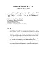
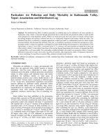
expectancy. A survival curve shows the relationship between the chance of survival
and the age of a population, and is calculated by cumulating the effects of annual death
rates over a lifetime. As shown in Figure 1, initially at age zero there is 100%
probability of survival; this decreases with increasing age as different causes of
mortality take their toll. Using this as the basis for calculations, the survival curves can
be calculated from hazard rates altered to take into account different mortality risks,
such as those associated with long-term exposure to pollution; this in turn will alter the
life expectancy of a population.

Any change in mortality patterns will then change the subsequent distribution of the
population. Differences between predicted survival curves can be used to quantify the
changes in life expectancy saved or lost by changes in the mortality rate and are
usually expressed in life years (or just ‘years’).

4

If we alter mortality rates, we alter survival curves and hence life expectancy. Life
expectancy of a birth cohort (a group of people born during a particular year or period)
is calculated by long-established arithmetical methods, from a series of mortality
hazard rates that are assumed to apply at different ages.

Figure 1 Typical shape of a survival curve showing the cumulative effect
of mortality risks on the probability of surviving to various ages.

2.2 AVAILABLE DATA
In order to calculate the mortality burden (number of attributable deaths) associated
with long term exposure to PM
2.5
in London, we need data on populations, deaths and
pollution concentrations. Files containing those data were supplied by the GLA,
sourced from the Data Management and Analysis Group, in line with the London Plan
projections.

Population projection data were provided for the years 2001-2031 inclusive, by sex,
and in 1-year age bands. With the exception of the City of London, they were given
separately by Borough, each broken down also by Ward, and given as ‘High’ and ‘Low’
projections. The ‘High’ population projections were used as a worse case scenario.
For City of London, there was no Ward breakdown. The City of London has a resident
population of less than 10,000 confined in a small geographic area.

Mortality data was represented by numbers of deaths, by sex and 5-year age group, for
the year 2008. The data were broken down by Borough, and were given as totals
(including non-neonatal total) and also by detailed cause-groups.

Modelled annual mean PM
2.5
concentrations were supplied for the years 2006, 2010
and 2015, with a value given for each Ward (including Wards within the City of
London). These total annual mean concentrations are made up of particles from human
and natural sources, as well as particles from sources outside London that have

travelled windborne into the area. Data for the year 2006 were used for the
Age
0 20 40 60 80 100 120
Survival probability
0.0
0.1
0.2
0.3
0.4
0.5
0.6
0.7
0.8
0.9
1.0
Age
0 20 40 60 80 100 120
Survival probability
0.0
0.1
0.2
0.3
0.4
0.5
0.6
0.7
0.8
0.9
1.0
5

calculations. (It should be noted that the base year for mortality data was for 2008 and
the annual mean PM
2.5
concentrations were for the year 2006.)


2.3 REORGANISATION OF DATA
Life-table calculations for scenarios in the future require age-specific mortality rates.
These were based on population projections in 2008 summarised at 5 year age groups.
Deaths used exclude the neonatal, i.e. those in the first month after birth.

Projections of total populations for males and females in 2008 were extracted for each
Ward
1
. From the file of estimated particulate concentrations, the mean annual PM
2.5

concentrations per ward for 2006 were extracted.


2.4 CALCULATIONS OF ATTRIBUTABLE DEATHS
Within each Borough in Greater London, a population-weighted mean PM
2.5

concentration was calculated, weighting the concentration for each Ward by its total
population
2
. From this, the corresponding proportional change in hazard rate was
computed (see Appendix A) and applied to the all-cause deaths for the Borough to

estimate attributable deaths corresponding to the mean concentration. These deaths
were then allocated to Wards in proportion to their total populations.

The main estimate used the coefficient recommended by COMEAP (2009), that there
is a 6% change in deaths from all causes for every 10 µg/m
3
change in average PM
2.5

concentrations. To inform sensitivity analysis, as recommended by COMEAP, the
calculations were repeated replacing the 6% figure with wide limits of 1% and 12%.
Details of the calculations are included in Appendix A.

2.5 LIFE-TABLE CALCULATIONS
IOM’s spreadsheet suite IOMLIFET was used to carry out life-table-based comparisons
of different imagined future scenarios, i.e. permanent and a one year reduction of 1
µg/m
3
of PM
2.5
in London. The baseline scenario assumed future age-specific mortality
rates based on the 2008 data for all London, calculated from all-cause death numbers,
excluding neonatal deaths, and the total population figures totalled over all Wards. The
IOMLIFET spreadsheets operate in 1-year age-groups, but deaths were available only
in five-year groups (plus <1 and the 4-year group 1-4). This was reconciled by
allocating the hazard rate for each age group to individual years within it.

Pollution impacts were calculated for scenarios representing both temporary reductions
in hazard for a single year, after which the hazards revert to their previous values; and
scenarios where the reduction is permanent. The notion that a change in pollution will

have an immediate effect is widely accepted as unrealistic. However, there are only
limited data to indicate over what timescale the benefits might accrue. This study has
made additional estimates adopting a time profile adopted by the US EPA for some of
their impact assessments. This models the phasing-in of the effects over 20 years as

1
A Ward breakdown was not available for the City of London
2
Since Ward populations were not available within the City of London, a Borough mean was
calculated unweighted.
6

30% in the first year, 12.5% in each of the next four years, and the final 20% phased in
gradually over years 6-20.

The life-table calculations were performed separately for males and females and then
combined. The impacts were very similar for both sexes, despite their known
differences in life expectancy. Estimates for other changes in PM
2.5
concentration can
be estimated, to a very good approximation, in direct proportion to the amount of
change.

Details of the calculations performed are included in Appendix B.
7

3 RESULTS
3.1 TOTAL ATTRIBUTABLE DEATHS
Table 1 shows the total population-weighted mean annual concentration of PM
2.5

(µg/m
3
) for Greater London, and implied attributable deaths, calculated as described
above, at concentration-response coefficients of 6%, 1% and 12% per 10µg/m
3
of
PM
2.5
. Totalled over Wards, the calculations predict a total of 4,267 attributable deaths
for the Greater London Area.

3.2 ATTRIBUTABLE DEATHS BY WARD
The table in Appendix C shows the estimates of population-weighted mean annual
PM
2.5
concentrations and attributable deaths per annum by Ward, based on the
mortality information supplied for 2008. In each ward, the estimate depends on the
size of the underlying population; on the annual number of deaths (which in turn will
depend partly on the local age distribution); and on the estimate of population-weighted
mean PM
2.5
concentration.

3.3 RESULTS OF LIFE-TABLE CALCULATIONS
Table 2 summarises the results of carrying out life-table calculations in IOMLIFET for
the whole population of London, and also for the extended population that includes new
births each year. A temporary elimination in one year of 1 µg/m
3
of PM

2.5
pollution is
predicted to save over 3,900 years of life in the current population, followed up to death
of the entire cohort over 106 years. If the reduction in pollution were permanent,
however, the total saving over that period would be over 400,000 life-years for the
current population, and over 600,000 when including new births. For the current
population, this is equivalent to an average 3 weeks per member of the 2008
population, with the gains differing by age.

8

Table 1 Population and population-weighted mean annual PM
2.5
(µg/m
3
) for Greater
London, and estimated attributable deaths (rounded to whole numbers) per annum
(based on 2008 rates), at concentration-response coefficients of 6%, 1% and 12% per
10µg/m
3
of PM
2.5
.


Area Area Total

PM
2.5

Attributable Deaths at coeff
t

Code

Popn

Conc

(change for 10 µg/m
3
PM
2.5
)



(µg/m
-3
)

6%

1%

12%

C000R
Greater
London
7,673,217

15.34

4,267

756

7,965



Table 2 Estimated total impacts on life expectancy (years) of changes in PM
2.5
air
pollution, for the current population of London in 2008 followed up through 2113, and
for the extended population including new births in that period.


Population
Reduction
in PM
2.5

Impact Pattern
2008 current

extended

1 1 year temporary 3,932

3,932

Permanent 421,430

614,496


20 year EPA phase in 405,659

598,333

9

4 DISCUSSION
The attributable deaths were estimated from data representing the actual mortality of
the population of London in 2008; they are the theoretical difference from a scenario in
which all-cause mortality is reduced by an amount related a certain reduction in annual
concentration of fine particulate matter, PM
2.5
. In a sense, they answer a question like
‘how many extra deaths can be attributed to current levels of PM
2.5

? However, a more
probing answer to this question would need to consider the temporal relationship
between the accumulation of exposure to PM and changes in mortality risk, because
the current level of risk may be due largely to e.g. gradual damage from past
exposures.

The term ‘attributable’ may itself cause some confusion. It is easy to see how this
technical term may imply to some readers that there are a number of deaths that are
directly (and solely) caused by, or attributed to, air pollution. However, the definition is
based purely on a comparison of two scenarios with different mortality risks, and could
reflect the situation where the risk to the whole populations differs by the same relative
amount. As an example, if we weight one side of a die so that the probability of
throwing a 6 is 1 in 5 rather than 1 in 6, then in say 600 throws we will get an average
of 1200 6s rather than the 1000 expected of a fair die. The changed probability
structure of the crooked die is responsible for 200 ‘attributable’ or extra 6s, but it is not
possible to identify the throws that produced the extra ones. We are simply comparing
the outcomes of two different risk structures, and thus it is with mortality scenarios in
humans. Levine (2007) overviews different possible uses of the ‘attributable’ concept,
depending on the context.

Here, it is unrealistic to believe that the estimated attributable deaths represent a
subset of deaths that are solely caused by PM
2.5
, while all remaining deaths were
unaffected by pollution. Since everyone breathes the air where they are, a more
realistic interpretation is that the risks are distributed across the whole population, with
a total mortality impact of the concentrations equivalent to that number of deaths. What
we do not know is exactly how the excess risk is distributed across the population;
whether the figure of 1.06 for 10µg/m
3

applies equally to all, or varies according to
factors either measurable or unseen and simply averages to this figure. One way or
another, we prefer the notion that air pollution affects everyone’s mortality risk to the
idea that there is a specific subset of individuals who are the only ones affected.

Here, the context of the ‘attributable’ deaths is that of comparing a baseline scenario
based on current (or very recent) mortality rates, with another where the rates have
been reduced by some impact factor. If we imagine that the response to changes in
pollution concentrations may not be immediate, then we may have to consider the
effects of a lag before the effects begin or before they are fully realised. The
calculation of deaths attributable to a particular concentration should then be
interpreted as relating to the unrealistic situation where that concentration has been
constant over the previous years.

The issue of lag in response to a change is important in considering policies to reduce
air pollution; it is an easy step from observing a concentration-response relationship in
cohort studies to imagining that eliminating or reducing the pollution source would
reduce death rates, but the speed with which this might happen will be a function of the
damage already done to individuals and their capacity for internal self-repair. A useful
analogy is with tobacco smoking, where it is known that following smoking cessation it
10

takes several years for risks in the ex-smoker to approach those of the lifelong non-
smoker.

It is fact that not all of measured PM
2.5
is man-made, and there is a portion that is from
the natural background and that cannot be controlled by policy or human action. In
addition, in current society the removal of all anthropogenic PM in a conurbation such

as London may not be considered a realistic goal. However, the life-year values given
in Table 3 for a 1µg/m
3
reduction in PM
2.5
concentrations could be scaled proportionally
to predict impacts for any smaller reductions envisaged. Predictions for changes down
to a PM
2.5
concentration of 7µg/m
3
remain within the range of the data from the ACS
study, while quantification to levels lower than this rest on the assumptions that the
same risk coefficient applies below this level and that there is no population threshold
to the relationship.

11

5 REFERENCES
Brunekreef B, Beelen R, Hoek G, Schouten L, Bausch-Goldbohm S, Fischer P,
Armstrong B, Hughes E, Jerrett M, van den Brandt P. (2009). Effects of long-term
exposure to traffic-related air pollution on respiratory and cardiovascular mortality in the
Netherlands: the NLCS-AIR study. Res Rep Health Eff Inst; 139: 5-71; discussion 73-
89.
Brunekreef B, Miller BG, Hurley F. (2007). The Brave New World of Lives Sacrificed &
Saved, and Deaths, Attributed To & Avoided. Epidemiology; 18: 785-788.
COMEAP. (2009). Long-Term Exposure to Air Pollution: Effect on Mortality. A report by
the Committee on the Medical Effects of Air Pollutants. London: Health Protection
Agency.
Hurley F, Hunt A, Cowie H, Holland M, Miller BG, Pye S, Watkiss P. (2005).

Methodology for the Cost-Benefit Analysis for CAFÉ: Volume 2: Health Impact
Assessment. Didcot, UK: AEA Technology Environment.
IGCB (2007) An Economic Analysis to inform the Air Quality Strategy. Volume 3.
Updated Third Report of the Interdepartmental Group on Costs and Benefits. London:
Department for the Environment, Food and Rural Affairs.
Krewski D, Jerrett M, Burnett RT, Ma R, Hughes E, Shi Y, Turner MC, Pope CA 3
rd
,
Thurston G, Calle EE, Thun MJ, Beckermann B, DeLuca P, Finkelstein N, Ito K, Moore
DK, Newbold KB, Ramsay T, Ross Z, Shin H, Tempalski MJ. (2009). Extended follow-
up and spatial analysis of the American Cancer Society study linking particulate air
pollution and mortality. Res Rep Health Eff Inst; 140: 5-144; discussion 115-36.
Levine B. (2007). What does the population attributable fraction mean? Prev Chronic
Dis [serial online]: 4; 1-5. www.cdc.gov/pcd/issues/2007/jan/06_0091.htm
Miller BG, Armstrong B. (2001). Quantification of the impacts of air pollution on chronic
cause-specific mortality. Edinburgh: Institute of Occupational Medicine. (IOM Report
TM/01/08).
Miller BG, Hurley JF (2006) Comparing estimated risks for air pollution with risks for
other health effects. Edinburgh: Institute of Occupational Medicine. (IOM Report
TM/06/01).
Miller BG, Hurley JF. (2003). Life table methods for quantitative impact assessments
in chronic mortality. Journal of Epidemiology and Community Health; 57: 200-206.
Miller BG. (2001). Predicting the impact of reduction in all-cause mortality rates. In:
DEFRA. (2001). An economic analysis to inform the review of the air quality strategy
objectives for particles: a second report of the Interdepartmental Group on Costs and
Benefits. London: Department for Environment, Food and Rural Affairs: 107-110.
Miller BG. (2001). Life-table methods for predicting and quantifying long-term impacts
on mortality. In : WHO (2001) Quantification of Health Effects of Exposure to Air
Pollution. Report on a WHO Working Group, Bilthoven, Netherlands, 20-22 November
2000. Copenhagen: WHO Regional Office for Europe.

12

Miller, B. (2003). Impact assessment of the mortality effects of longer-term exposure to
air pollution: exploring cause-specific mortality and susceptibility. Edinburgh: Institute of
Occupational Medicine. (IOM Report TM/03/01).
Pope CA 3rd, Burnett RT, Thun MJ, Calle EE, Krewski D, Ito K, Thurston GD. (2002).
Lung cancer, cardiopulmonary mortality, and long-term exposure to fine particulate air
pollution. JAMA; 287:132-1141.
WHO. (2000). Quantification of the health effects of exposure to air pollution. Bonn:
World Health Organization, European Centre for Environment and Health.
Woodruff TJ, Grillo J, Schoendorf KC. (1997). The Relationship between selected
causes of post neonatal infant mortality and particulate air pollution in the United
States. Env Health Persp; 105: 608-612.

13

APPENDIX A: CALCULATION OF ATTRIBUTABLE DEATHS

The core estimate of concentration-response recommended by COMEAP is a 6%
change in all-cause mortality hazard per 10µg/m
3
change in mean airborne PM
2.5

concentration. If we extend this to associate a change in mortality with the entirety of a
geographically specific mean concentration x, in the knowledge that this coefficient
came from a study that fitted its response to the logarithm of exposure, then the relative
risk for the impact scales to

rr(x) = (1.06)

x/10


Relative risks were calculated in this way from x=mean PM
2.5
concentration for each
Borough.

From a relative risk, the attributable fraction of deaths corresponding to a concentration
of x is given by

f
attr
= (1 – 1/rr(x))

This was calculated for each Borough, and multiplied by the total deaths in that
Borough to estimate a figure for attributable deaths corresponding to a mean
concentration x. Finally, the total attributable deaths for each Borough were allocated
to their constituent Wards in proportion to the total population of each Ward.


The reorganisation, summarising and calculation were carried out using a mixture of
the facilities of the MS Excel software and the statistical package Genstat.

14

15

APPENDIX B: LIFE TABLE CALCULATIONS

In the context of a health impact assessment, we make further assumptions, e.g. that
some policy change will affect the future mortality rates. We can then compare the
survival curves for two scenarios, calculated with and without the policy impact, and the
difference in life expectancy is a measure of the impact. For a defined cohort, the
temporal patterns of deaths under the baseline (no change) and impacted scenarios
will differ, as will the total life expectancy implied. The difference in the number of
deaths expected each year can be displayed graphically. However, the total deaths
over a lifetime follow-up must be the same as the initial size of the cohort, so there are
no ‘saved’ deaths overall (Brunekreef et al, 2007).

Assessing the impact on a current population, we need to take into account that they
have a distribution of ages. Miller and Hurley (2003, 2006) showed in detail how this
could be accommodated within standard spreadsheet packages. A two-dimensional
array is constructed, indexed by both age and calendar year, and life-table calculations
are performed for every age-specific sub-cohort, down diagonals of the array. If this is
done for two scenarios one baseline and another representing the impact of some
change, then the results of the change can be compared. Using spreadsheets means
that there is great flexibility in summarising the results. For each age-year
combination, there are available estimates of expected deaths and survivors, from
which can be derived the total person-years (or ‘life-years’) contributed. Summary
figures, tables or graphical displays can be constructed in numerous ways. Just as for
a single cohort, comparison of the patterns of deaths in two scenarios applying to a
current population may redistribute their expect pattern in time, but the eventual total
numbers of deaths must be the same. (This will not be the case, however, if we
summarise the impact over an extended population comprising the current population
and future birth cohorts).

The IOMLIFET system allows for complete flexibility in how impacts are assumed to
affect future mortality hazard rates; these can be manipulated over any combination of
age and calendar year. We have calculated the effect of a change in hazard rates

corresponding to a reduction in air pollution of just 1 µg/m
3
, which gives

(1.06)
-1/10
= 0.994190

It would be possible to repeat these calculations for a change equal to the population-
weighted average over London, 15.34 µg/m
3
. This yields a mortality impact factor

(1.06)
-15.34/10
= 0.914494

Theoretical and empirical evidence, however, shows that the impact in life-years scales
very nearly with the amount of change in the mean concentration, so estimates for
other changes may, to a very good approximation, be obtained by proportional scaling
based on the result for 1 µg/m
3
.
16

17

APPENDIX C: ESTIMATES OF ATTRIBUTABLE DEATHS
Populations and population weighted mean annual PM
2.5

(µg/m
3
) by Ward and
estimated attributable deaths (rounded to whole numbers) per annum, based on 2008
rates, at COMEAP’s recommended concentration-response coefficient of 6% per
10µg/m
3
of PM
2.5
, plus estimates at limits of 1% and 12% to inform sensitivity analysis.


Area Area Total

PM
2.5

Attributable Deaths at coeff
t

Code

Popn

Conc

(change for 10 µg/m
3
PM
2.5

)



(µg/m
3
)

6%

1%

12%








C000R
Greater London
7,673,217

15.34

4,267

756

7,965








H00AA
City of London
9155

17.59

4

1

7

Ward





00ABFX Abbey 11,558

15.39

8

1

15

00ABFY Alibon 9,876

14.86

7

1

13

00ABFZ Becontree 11,716

14.94

8

1

15

00ABGA Chadwell Heath 9,470

14.80

7

1

12

00ABGB Eastbrook 10,478

14.66

7

1

13

00ABGC Eastbury 10,390

15.25

7

1

13

00ABGD Gascoigne 10,721

15.62

7

1

14

00ABGE Goresbrook 11,036

15.16

8

1

14

00ABGF Heath 9,852

14.84

7

1

13

00ABGG Longbridge 9,604

15.03

7

1

12

00ABGH Mayesbrook 9,658

14.91

7

1

12

00ABGJ Parsloes 9,170

14.94

6

1

12

00ABGK River 10,678

15.09

7

1

14

00ABGL Thames 9,493

15.31

7

1

12

00ABGM Valence 8,841

14.95

6

1

11

00ABGN Village 10,027

14.75

7

1

13

00ABGP Whalebone 9,789

14.99

7

1

13

00ACFX Brunswick Park 15,577

14.87

10

2

18

00ACFY Burnt Oak 15,672

14.89

10

2

18

00ACFZ Childs Hill 18,103

15.51

11

2

21

00ACGA Colindale 15,804

15.06

10

2

18

00ACGB Coppetts 15,036

15.31

9

2

17

00ACGC East Barnet 15,805

14.67

10

2

18

00ACGD East Finchley 15,019

15.34

9

2

17

00ACGE Edgware 15,253

14.87

9

2

18

00ACGF Finchley Church End 14,652

15.43

9

2

17

00ACGG Garden Suburb 15,064

15.29

9

2

17

00ACGH Golders Green 16,787

15.81

10

2

19

00ACGJ Hale 16,088

15.00

10

2

18

00ACGK Hendon 15,973

15.52

10

2

18

00ACGL High Barnet 14,762

14.62

9

2

17

00ACGM Mill Hill 17,036

14.95

10

2

20

00ACGN Oakleigh 15,224

14.84

9

2

17

00ACGP Totteridge 14,880

14.70

9

2

17

00ACGQ Underhill 15,996

14.64

10

2

18

00ACGR West Finchley 14,960

15.12

9

2

17

00ACGS West Hendon 14,977

15.66

9

2

17

18

Area Area Total

PM
2.5

Attributable Deaths at coeff
t

Code

Popn

Conc

(change for 10 µg/m
3
PM
2.5
)



(µg/m
3
)

6%

1%

12%








00ACGT Woodhouse 16,084

15.17

10

2

18

00ADGA Barnehurst 10,177

14.80

7

1

14

00ADGB Belvedere 10,920

14.76

8

1

15

00ADGC Blackfen and Lamorbey 10,341

14.80

8

1

14

00ADGD Blendon and Penhill 10,319

15.04

8

1

14

00ADGE Brampton 10,249

14.76

7

1

14

00ADGF Christchurch 10,403

15.01

8

1

14

00ADGG Colyers 10,525

14.74

8

1

14

00ADGH Crayford 10,306

14.90

7

1

14

00ADGJ Cray Meadows 10,321

14.68

8

1

14

00ADGK Danson Park 10,303

14.99

7

1

14

00ADGL East Wickham 10,283

14.84

7

1

14

00ADGM Erith 10,596

14.86

8

1

14

00ADGN Falconwood and Welling 10,503

15.09

8

1

14

00ADGP Lesnes Abbey 10,882

14.81

8

1

15

00ADGQ Longlands 9,705

15.01

7

1

13

00ADGR North End 10,496

14.73

8

1

14

00ADGS Northumberland Heath 10,548

14.74

8

1

14

00ADGT St. Mary's 9,999

14.81

7

1

14

00ADGU St. Michael's 10,569

14.77

8

1

14

00ADGW Sidcup 10,360

14.81

8

1

14

00ADGX Thamesmead East 11,140

14.76

8

1

15

00AEGJ Alperton 12,643

15.29

6

1

11

00AEGK Barnhill 13,204

15.11

6

1

12

00AEGL Brondesbury Park 12,299

15.44

6

1

11

00AEGM Dollis Hill 12,677

15.75

6

1

11

00AEGN Dudden Hill 14,058

15.83

7

1

13

00AEGP Fryent 12,264

15.04

6

1

11

00AEGQ Harlesden 13,216

15.72

6

1

12

00AEGR Kensal Green 11,340

15.89

5

1

10

00AEGS Kenton 12,163

14.91

6

1

11

00AEGT Kilburn 14,744

15.71

7

1

13

00AEGU Mapesbury 14,242

15.44

7

1

13

00AEGW Northwick Park 12,518

14.99

6

1

11

00AEGX Preston 14,061

15.07

7

1

13

00AEGY Queens Park 13,157

15.61

6

1

12

00AEGZ Queensbury 14,272

14.93

7

1

13

00AEHA Stonebridge 17,229

15.78

8

1

16

00AEHB Sudbury 12,884

15.13

6

1

12

00AEHC Tokyngton 12,169

15.36

6

1

11

00AEHD Welsh Harp 12,726

15.59

6

1

11

00AEHE Wembley Central 11,712

15.18

6

1

11

00AEHF Willesden Green 14,285

15.51

7

1

13

00AFGD Bickley 14,362

14.77

10

2

19

00AFGE Biggin Hill 10,353

14.37

7

1

14

00AFGF Bromley Common and Keston 14,375

14.62

10

2

19

00AFGG Bromley Town 15,656

14.94

11

2

21

00AFGH Chelsfield and Pratts Bottom 14,903

14.42

11

2

20

00AFGJ Chislehurst 15,137

14.72

11

2

20

00AFGK Clock House 16,107

14.96

12

2

22

19

Area Area Total

PM
2.5

Attributable Deaths at coeff
t

Code

Popn

Conc

(change for 10 µg/m
3
PM
2.5
)



(µg/m
3
)

6%

1%

12%








00AFGL Copers Cope 15,098

14.94

11

2

20

00AFGM Cray Valley East 14,960

14.51

11

2

20

00AFGN Cray Valley West 16,109

14.66

12

2

22

00AFGP Crystal Palace 11,517

15.07

8

1

16

00AFGQ Darwin 4,846

14.36

3

1

7

00AFGR Farnborough and Crofton 14,192

14.55

10

2

19

00AFGS Hayes and Coney Hall 14,888

14.61

11

2

20

00AFGT Kelsey and Eden Park 15,541

14.86

11

2

21

00AFGU Mottingham and Chislehurst North 10,277

14.83

7

1

14

00AFGW Orpington 15,295

14.54

11

2

21

00AFGX Penge and Cator 16,891

14.99

12

2

23

00AFGY Petts Wood and Knoll 13,593

14.56

10

2

18

00AFGZ Plaistow and Sundridge 14,622

14.80

11

2

20

00AFHA Shortlands 9,419

14.82

7

1

13

00AFHB West Wickham 14,323

14.75

10

2

19

00AGGD Belsize 11,991

15.86

6

1

12

00AGGE Bloomsbury 9,205

17.54

5

1

9

00AGGF Camden Town with Primrose Hill 12,286

16.21

6

1

12

00AGGG Cantelowes 11,220

16.53

6

1

11

00AGGH Fortune Green 10,895

15.70

6

1

10

00AGGJ Frognal and Fitzjohns 11,937

15.73

6

1

11

00AGGK Gospel Oak 10,817

15.85

6

1

10

00AGGL Hampstead Town 11,016

15.49

6

1

11

00AGGM Haverstock 11,749

15.88

6

1

11

00AGGN Highgate 10,622

15.29

5

1

10

00AGGP Holborn and Covent Garden 11,438

17.18

6

1

11

00AGGQ Kentish Town 12,424

15.99

6

1

12

00AGGR Kilburn 11,000

15.88

6

1

11

00AGGS King's Cross 11,717

17.19

6

1

11

00AGGT Regent's Park 12,324

16.70

6

1

12

00AGGU St. Pancras and Somers Town 13,081

16.74

7

1

13

00AGGW Swiss Cottage 12,409

15.84

6

1

12

00AGGX West Hampstead 11,067

15.84

6

1

11

00AHGE Addiscombe 16,076

15.08

10

2

18

00AHGF Ashburton 13,905

14.93

8

1

16

00AHGG Bensham Manor 16,857

15.08

10

2

19

00AHGH Broad Green 15,794

15.38

9

2

18

00AHGJ Coulsdon East 12,092

14.49

7

1

14

00AHGK Coulsdon West 13,412

14.80

8

1

15

00AHGL Croham 15,043

14.99

9

2

17

00AHGM Fairfield 16,149

15.16

10

2

18

00AHGN Fieldway 11,019

14.55

7

1

12

00AHGP Heathfield 12,984

14.66

8

1

15

00AHGQ Kenley 14,240

14.62

9

2

16

00AHGR New Addington 10,261

14.48

6

1

11

00AHGS Norbury 14,632

15.09

9

2

16

00AHGT Purley 14,111

15.00

8

1

16

00AHGU Sanderstead 12,078

14.62

7

1

14

00AHGW Selhurst 15,175

15.17

9

2

17

00AHGX Selsdon and Ballards 11,751

14.63

7

1

13