Enhancement of Local Air Pollution by Urban CO2 Domes docx
Bạn đang xem bản rút gọn của tài liệu. Xem và tải ngay bản đầy đủ của tài liệu tại đây (492.11 KB, 6 trang )
Enhancement of Local Air Pollution
by Urban CO
2
Domes
MARK Z. JACOBSON*
Department of Civil and Environmental Engineering, Stanford
University, Stanford, California 94305-4020
Received October 3, 2009. Revised manuscript received
December 21, 2009. Accepted March 2, 2010.
Data suggest that domes of high CO
2
levels form over cities.
Despite our knowledge of these domes for over a decade, no
study has contemplated their effects on air pollution or
health. In fact, all air pollution regulations worldwide assume
arbitrarily that such domes have no local health impact, and carbon
policy proposals, such as “cap and trade”, implicitly assume
that CO
2
impacts are the same regardless of where emissions
occur. Here, it is found through data-evaluated numerical
modeling with telescoping domains from the globe to the U.S.,
California, and Los Angeles, that local CO
2
emissions in
isolation may increase local ozone and particulate matter.
Although health impacts of such changes are uncertain, they
are of concern, and it is estimated that that local CO
2
emissions
may increase premature mortality by 50-100 and 300-1000/
yr in California and the U.S., respectively. As such, reducing
locally emitted CO
2
may reduce local air pollution mortality
even if CO
2
in adjacent regions is not controlled. If correct, this
result contradicts the basis for air pollution regulations
worldwide, none of which considers controlling local CO
2
based on its local health impacts. It also suggests that a “cap
and trade” policy should consider the location of CO
2
emissions,
as the underlying assumption of the policy is incorrect.
Introduction
Although CO
2
is generally well-mixed in the atmosphere,
data indicate that its mixing ratios are higher in urban than
in background air, resulting in urban CO
2
domes (1–6).
Measurements in Phoenix, for example, indicate that peak
and mean CO
2
in the city center were 75%and38-43% higher,
respectively, than in surrounding rural areas (2). Recent
studies have examined the impact of global greenhouse gases
on air pollution (7–13). Whereas one study used a 1-D model
to estimate the temperature profile impact of a CO
2
dome
(3), no study has isolated the impact of locally emitted CO
2
on air pollution or health. One reason is that model
simulations of such an effect require treatment of meteo-
rological feedbacks to gas, aerosol, and cloud changes, and
few models include such feedbacks in detail. Second, local
CO
2
emissions are close to the ground, where the temperature
contrast between the Earth’s surface and thelowestCO
2
layers
is small. However, studies have not considered that CO
2
domes result in CO
2
gradients high above the surface. If locally
emitted CO
2
increases local air pollution, then cities, counties,
states, and small countries can reduce air pollution health
problems by reducing their own CO
2
emissions, regardless
of whether other air pollutants are reduced locally or whether
other locations reduce CO
2
.
Methodology and Evaluation
For this study, the nested global-through-urban 3-D model,
GATOR-GCMOM (13–17) was used to examine the effects
of locally emitted CO
2
on local climate and air pollution.
A nested model is one that telescopes from a large scale
to more finely resolved domains. The model and its
feedbacks are described in the Supporting Information.
Example CO
2
feedbacks treated include those to heating
rates thus temperatures, which affect (a) local temperature
and pressure gradients, stability, wind speeds, cloudiness,
and gas/particle transport, (b) water evaporation rates,
(c) the relative humidity and particle swelling, and (d)
temperature-dependent natural emissions, air chemistry,
and particle microphysics. Changes in CO
2
also affect (e)
photosynthesis and respiration rates, (f) dissolution and
evaporation rates of CO
2
into the ocean, (g) weathering
rates, (h) ocean pH and chemical composition, (i) sea spray
pH and composition, and (j) rainwater pH and composi-
tion. Changes in sea spray composition, in turn, affect sea
spray radiative properties, thus heating rates.
The model was nested from the globe (resolution
4°SN×5°WE) to theU.S.(0.5°×0.75°), California (0.20°×0.15°),
and Los Angeles (0.045°×0.05°). The global domain included
47 sigma-pressure layers up to 0.22 hPa (∼60 km), with high
resolution (15 layers) in the bottom 1 km. The nested regional
domains included 35 layers exactly matching the global layers
up to 65 hPa (∼18 km). The model was initialized with
1-degree global reanalysis data (18) but run without data
assimilation or model spinup.
Three original pairs of baseline and sensitivity simulations
were run: one pair nested from the globe to California for
one year (2006), one pair nested from the globe to California
to Los Angeles for two sets of three months (Feb-Apr, Aug-
Oct, 2006), and one pair nested from the globe to the U.S.
for two sets of three months (Jan-Mar, Jul-Sep, 2006). The
seasonal periods were selected to obtain roughly winter/
summer results that could be averaged to estimate annual
values. A second 1-year (2007) simulation pair was run for
California to test interannual variability. In each sensitivity
simulation, only anthropogenic CO
2
emissions (emCO
2
) were
removed from the finest domain. Initial ambient CO
2
was
the same in all domains of both simulations, and emCO
2
was
the same in the parent domains of both. As such, all resulting
differences were due solely to initialchangesinlocallyemitted
(in the finest domain) CO
2
.
The model and comparisons with data have been de-
scribed in over 50 papers, including recently (13–17). Figure
1 further compares modeled O
3
,PM
10
, and CH
3
CHO from
August 1-7 of the baseline (with emCO
2
) and sensitivity (no
emCO
2
) simulations from the Los Angeles domain with data.
The comparisons indicate good agreement for ozone in
particular. Since emCO
2
was the only variable that differed
initially between simulations, it was theinitiatingcausalfactor
in the increases in O
3
,PM
10
, and CH
3
CHO seen in Figure 1.
Although ozone was predicted slightly better in t he no-emCO
2
case than in the emCO
2
case during some hours, modeled
ozone in the emCO
2
case matched peaks better by about
0.5% averaged over comparisons with all data shown and
not shown.
Results
Figure 2a,b shows the modeled contribution of California’s
CO
2
emissions to surface and column CO
2
, respectively,
averaged over a year. The CO
2
domes over Los Angeles, the
San Francisco Bay Area, Sacramento (38.58 N, 121.49 W),
* Corresponding author phone: (650)723-6836; e-mail:
Environ. Sci. Technol. 2010, 44, 2497–2502
10.1021/es903018m 2010 American Chemical Society VOL. 44, NO. 7, 2010 / ENVIRONMENTAL SCIENCE & TECHNOLOGY
9
2497
Published on Web 03/10/2010
and the Southern Central Valley are evident. The largest
surface CO
2
increase (5%, or 17.5 ppmv) was lower than
observed increases in cities (2) since the resolution of the
California domain was coarser than the resolution of
measurements. As shown below for Los Angeles, an increase
in model resolution increases the magnitude of the surface
and column CO
2
dome.
Population-weighted (PW) and domain-averaged (DA)
changes in several parameters can help to elucidate the
effects of the CO
2
domes. A PW value is the product of a
parameter value and population in a grid cell, summed
over all grid cells, all divided by the summed population
among all cells. Thus, a PW value indicates changes
primarily in populated areas, whereas a DA value indicates
changes everywhere, independent of population. The PW
and DA increases in surface CO
2
due to emCO
2
were 7.4
ppmv and 1.3 ppmv, respectively, but the corresponding
increases in column CO
2
were 6.0 g/m
2
and 1.53 g/m
2
,
respectively, indicating, along with Figure 2a,b, that
changes in column CO
2
were spread horizontally more
than were changes in surface CO
2
. This is because surface
winds are usually slower than winds aloft, so only when
surface CO
2
mixes vertically is it transported much
horizontally, and when that occurs, surface CO
2
is quickly
replenished with new emissions.
The CO
2
increases in California increased the PW air
temperature by about 0.0063 K, more than it changed the
domain-averaged air temperature (+0.00046) (Figure 2c).
Thus, CO
2
domes had greater temperature impacts where
the CO
2
was emitted and where people lived than in the
domain average. This result held for the effects of emCO
2
on column water vapor (Figure 2d - PW: +4.3 g/m
2
; DA:
+0.88 g/m
2
), ozone (Figure 2e - PW: +0.06 ppbv; DA:
+0.0043 ppbv), PM
2.5
(Figure 2g - PW: +0.08 µg/m
3
;
DA: -0.0052 µg/m
3
), and PAN (Figure 2i - PW: +0.002 ppbv;
DA: -0.000005 ppbv). The peak surface air temperature
increases in Figure 2c (and in the Los Angeles simulations)
were ∼0.1 K, similar to those found from 1-D radiative
only calculations for Phoenix (3). Peak ozone and its health
effects occurred over Los Angeles and Sacramento (Figure
2e,f), where increases in CO
2
(Figure 2a), temperature
(although small for Sacramento, Figure 2c), and column
H
2
O (Figure 2d) occurred.
Figure 3 elucidates spatial correlations between annually
averaged changes in local ambient CO
2
caused by emCO
2
and changes in other parameters. Increases in temperature,
water vapor, and ozone correlated positively and with
statistical significance (p <<0.05) with increases in CO
2
.
Ozone increases also correlated positively and with strong
significance with increases in water vapor and temperature.
A previous study found that increases in temperature and
water vapor both increase ozone at high ozone but cause
little change in ozone at low ozone (13), consistent with this
result.
PM
2.5
correlated slightly negatively (r ) 0.017) but without
statistical significance, with higher temperature and much
more positively (r ) 0.23) and with strong significance (p
< 0.0001) with higher water vapor in California. Higher
temperature decreased PM
2.5
by increasing vapor pressures
thus PM evaporation and by enhancing precipitation in
some locations. Some PM
2.5
decreases with higher tem-
perature were offset by biogenic organic emission increases
with higher temperatures followed by biogenic oxidation
to organic PM. But, in populated areas of California,
biogenic emissions are relatively low. Some PM
2.5
decreases
were also offset by surface PM
2.5
increases caused by slower
surface winds due to enhanced boundary-layer stability
from CO
2
, which reduced the downward transport of fast
winds aloft to the surface (13). While higher temperature
slightly decreased PM
2.5
, higher water vapor due to emCO
2
increased PM
2.5
by increasing aerosol water content,
increasing nitric acid and ammonia gas dissolution,
forming more particle nitrate and ammonium. Higher
ozone from higher water vapor also increased oxidation
of organic gases to organic PM. Overall, PM
2.5
increased
with increasing CO
2
, but because of the opposing effects
of temperature and water vapor on PM
2.5
, the net positive
correlation was weak (r ) 0.022) and not statistically
significant (p ) 0.17). However, when all CO
2
increases
below 1 ppmv were removed, the correlation improved
substantially (r ) 0.047, p ) 0.07). Further, the correlation
was strongly statistically significant for Los Angeles and
U.S. domains, as discussed shortly.
Health effect rates (y) due to pollutants in each model
domain for each simulation were determined from
where x
i,t
is the concentration in grid cell i at time t, x
th
is the
threshold concentration below which no health effect occurs,
β is the fractional increase in risk per unit x, y
0
is the baseline
health effect rate, and P
i
is the grid cell population. Table 1
provides sums or values of P, β, y
0
, and x
th
. Differences in
health effects between two simulations were obtained by
differencing the aggregated effects from each simulation
determined from eq 1. The relationship between ozone
exposure and premature mortality is uncertain; however, ref
19 suggests that it is “highly unlikely” to be zero. Similarly,
ref 20 suggests that the exact relationship between PM
2.5
exposure and mortality is uncertain but “likely causal”.
Cardiovascular effects of PM
2.5
are more strongly “causal”.
Although health effects of PM
2.5
differ for different chemical
components within PM
2.5
, almost all epidemiological studies
FIGURE 1. Paired-in-time-and-space comparisons of modeled
baseline (solid lines), modeled no-emCO
2
(dashed lines), and data
(22) (dots) for ozone, sub-10-µm particle mass, and acetaldehyde
from the Los Angeles domain for August 1-7, 2006 of the Aug-Oct
2006 simulation. Local standard time is GMT minus 8 h.
y ) y
0
∑
i
{
P
i
∑
t
(1 - exp[-β × max(x
i,t
- x
th
, 0)])
}
(1)
2498
9 ENVIRONMENTAL SCIENCE & TECHNOLOGY / VOL. 44, NO. 7, 2010
correlating particle changes with health use ambient PM
2.5
measurements to derive such correlations. For consistency,
it is therefore necessary to apply β values from such studies
to modeled PM
2.5
(22).
California’s local CO
2
resulted here in ∼13 (with a range
of 6-19 due to uncertainty in epidemiological data)
additional ozone-related premature mortalities/year (Fig-
ure 2f) or 0.3% above the baseline 4600 (2300-6900)/year
(Table 1). Higher PM
2.5
due to emCO
2
contributed another
∼39 (13-60) premature mortalities/year (Figure 2h), 0.2%
above the baseline rate of 22,500 (5900-42,000)/year.
Changes in cancer due to emCO
2
were relatively small
(Table 1). Additional uncertainty arises due to the model
itself and interannual variations in concentration. Some
of the model uncertainties are elucidated in comparisons
with data, such as in Figure 1; however, it is difficult to
translate such uncertainty into mortality uncertainty.
Interannual variations in concentrations were examined
by running a second pair of simulations for California,
starting one year after the first. The results of this simulation
FIGURE 2. Modeled annually averaged difference for several surface or column (if indicated) parameters in California, parts of
Nevada, and parts of New Mexico when two simulations (with and without emCO
2
) were run. The numbers in parentheses are
average population-weighted changes for the domain shown.
FIGURE 3. Scatter plots of paired-in-space one-year-averaged changes between several parameter pairs, obtained from all
near-surface grid cells of the California domain. Also shown is an equation for the linear fit through the data points in each case
and the r and p values for the fits. The equation describes correlation only, not cause and effect, between each parameter pair.
VOL. 44, NO. 7, 2010 / ENVIRONMENTAL SCIENCE & TECHNOLOGY
9 2499
were similar to those for the first, with ∼51 (17-82)
additional ozone- plus PM
2.5
-related premature mortali-
ties/year attributable to emCO
2
.
Simulations for Los Angeles echo results for California
but allowed for a more resolved picture of the effects of
emCO
2
. Figure 4a (Feb-Apr) indicates that the near-surface
CO
2
dome that formed over Los Angeles peaked at about 34
ppmv, twice that over the coarser California domain. The
column difference (Figure 4b) indicates a spreading of the
dome over a larger area than the surface dome. In Feb-Apr
and Aug-Oct, emCO
2
enhanced PW ozone and PM
2.5
,
increasing mortality (Figure 4, Table 1) and other health
effects (Table 1). The causes of such increases, however,
differed with season.
During Feb-Apr, infrared absorption by emCO
2
warmed
air temperatures (Figure 4c) up to ∼3 km altitude, increasing
the land-ocean temperature gradient by about 0.2 K over 50
km, increasing surface sea-breeze wind speeds by ∼0.06
m/s, and increasing water vapor transport to and soil-water
evaporation in Los Angeles (Figure 4d). Higher temperatures
and water vapor slightly increased ozone and PM
2.5
for the
reasons given in ref 13. The high wind speeds also increased
resuspension of road and soil dust and moved PM more to
the eastern basin.
During summer, Los Angeles boundary layer heights,
temperature inversions, land-sea temperature gradients, sea
breeze wind speeds, water evaporation rates, column water
vapor, and stratus cloud formation are greater than in
summer. Since boundary-layer heights were higher during
the Aug-Oct simulations, CO
2
mixed faster up to higher
altitudes during summer. Initially, the higher CO
2
warmed
the air up to 4 km above topography, but the higher
TABLE 1. Summary of Locally-Emitted CO
2
’s (emCO
2
) Effects on Cancer, Ozone Mortality, Ozone Hospitalization, Ozone
Emergency-Room (ER) Visits, and Particulate-Matter Mortality in California (CA), Los Angeles (LA), and the United States (U.S.)
d
annual base CA base minus no emCO
2
CA annual base LA
base minus
no emCO
2
LA annual base U.S.
base minus
no emCO
2
U.S.
ozone g 35 ppbv (ppbv) 47.4 +0.060 44.7 +0.12 47.0 +0.044
PM
2.5
(µg/m
3
) (pop-weight) 50.0 +0.08 36 +0.29 64.4 +0.041
PM
2.5
(µg/m
3
) (all land) 21.5 -0.007 25.8 +0.06 32.8 +0.039
formaldehyde (ppbv) 4.43 +0.0030 4.1 +0.054 6.75 +0.066
acetaldehyde (ppbv) 1.35 +0.0017 1.3 +0.021 2.45 +0.016
1,3-butadiene (ppbv) 0.11 -0.00024 0.23 +0.0020 0.077 +0.0005
benzene (ppbv) 0.30 -0.00009 0.37 +0.0041 0.34 +0.020
Cancer
USEPA cancers/yr
a
44.1 0.016 22.0 +0.28 573 +6.9
OEHHA cancers/yr
a
54.4 -0.038 37.8 +0.39 561 +11.8
Ozone Health Effects
high O
3
mortalities/yr
b
6860 +19 2140 +20 52,300 +245
med. O
3
mortalities/yr
b
4600 +13 1430 +14 35,100 +166
low O
3
mortalities/yr
b
2300 +6 718 +7 17,620 +85
O
3
hospitalizations/yr
b
26,300 +65 8270 +75 200,000 +867
ozone ER visits/yr
b
23,200 +56 7320 +66 175,000 +721
PM Health Effects
high PM
2.5
mortalities/yr
c
42,000 +60 16,220 +147 44,800 +810
med. PM
2.5
mortalities/yr
c
22,500 +39 8500 +81 169,000 +607
low PM
2.5
mortalities/yr
c
5900 +13 2200 +22 316,000 +201
a
USEPA (U.S. Environmental Protection Agency) and OEHHA (Office of Environmental Health Hazard Assessment)
cancers/yr were found by summing, over all model surface grid cells and the four carcinogens (formaldehyde,
acetaldehyde, 1,3-butadiene, and benzene), the product of individual CUREs (cancer unit risk estimates)increased 70-year
cancer risk per µg/m
3
sustained concentration change), the mass concentration (µg/m
3
) (for baseline statistics) or mass
concentration difference (for difference statistics) of the carcinogen, and the population in the cell and then dividing by the
population of the model domain and by 70 yr. USEPA CURES were 1.3 × 10
-5
(formaldehyde), 2.2 × 10
-6
(acetaldehyde),
3.0 × 10
-5
(butadiene), 5.0 × 10
-6
()average of 2.2 × 10
-6
and 7.8 × 10
-6
) (benzene) (www.epa.gov/IRIS/). OEHHA CUREs
were 6.0 × 10
-6
(formaldehyde), 2.7 × 10
-6
(acetaldehyde), 1.7 × 10
-4
(butadiene), 2.9 × 10
-5
(benzene)
(www.oehha.ca.gov/risk/ChemicalDB/index.asp).
b
High, medium, and low mortalities/yr, hospitalizations/yr, and
emergency-room (ER) visits/yr due to short-term O
3
exposure were obtained from eq 1, assuming a threshold (x
th
)of35
ppbv (23). The baseline 2003 U.S. mortality rate (y
0
) was 833 mortalities/yr per 100,000 (24). The baseline 2002
hospitalization rate due to respiratory problems was 1189 per 100,000 (25). The baseline 1999 all-age emergency-room visit
rate for asthma was 732 per 100,000 (26). The fractional increases (β) in the number of premature mortalities from all
causes due to ozone were 0.006, 0.004, and 0.002 per 10 ppbv increase in daily 1-h maximum ozone (27). These were
multiplied by 1.33 to convert the risk associated with a 10 ppbv increase in 1-h maximum O
3
to that associated with a 10
ppbv increase in 8-h average O
3
(23). The central value of the increased risk of hospitalization due to respiratory disease
was 1.65% per 10 ppbv increase in 1-h maximum O
3
(2.19% per 10 ppbv increase in 8-h average O
3
), and that for all-age ER
visits for asthma was 2.4% per 10 ppbv increase in 1-h O
3
(3.2% per 10 ppbv increase in 8-h O
3
)(25, 26).
c
The mortality
rate due to long-term PM
25
exposure was calculated from eq 1. Increased premature mortality risks to those g30 years
were 0.008 (high), 0.004 (medium), and 0.001 (low) per 1 µg/m
3
PM
2.5
> 8 µg/m
3
based on 1979-1983 data (28). From 0-8
µg/m
3
, the increased risks were assumed to be a quarter of the risks for those >8 µg/m
3
to account for reduced risk near
zero PM
2.5
(13). The all-cause 2003 U.S. mortality rate of those g30 years was 809.7 mortalities/yr per 100,000 total
population. Reference 29 provides higher relative risks of PM
2.5
health effects data; however, the values from ref 28 were
retained to be conservative.
d
Results are shown for the with-emCO
2
emissions simulation (“base”) and the difference
between the base and no emCO
2
emissions simulations (“base minus no-emCO
2
”) for each case. The domain summed
populations (sum of P
i
in eq 1) in the CA, LA, and U.S. domains were 35.35 million, 17.268 million, and 324.07 million,
respectively. All concentrations except the second PM
2.5
, which is an all-land average, were near-surface values weighted
spatially by population. PM
2.5
concentrations in the table include liquid water, but PM
2.5
used for health calculations were
dry. CA results were for an entire year, LA results were an average of Feb-Apr and Aug-Oct (Figure 4), and U.S. results
were an average of Jan-Mar and Jul-Sep.
2500
9 ENVIRONMENTAL SCIENCE & TECHNOLOGY / VOL. 44, NO. 7, 2010
temperatures from 1.5-4 km decreased the upper-level sea-
breeze return flow (figures not shown) decreased pressure
aloft, reducing the flow of moisture from land to ocean aloft
(increasing it from ocean to land), increasing cloud optical
depth over land by up to 0.4-0.6 optical depth units,
decreasing summer surface solar radiation by at most 3 -4
W/m
2
locally, decreasing local ground temperatures by up
to 0.2 K (Figure 4g) while retaining the warmer air aloft. The
excess water vapor aloft over land mixed to the surface (Figure
4h), increasing ozone (which increases chemically with water
vapor at high ozone) and the relative humidity, which
increased aerosol particle swelling, increasing gas growth
onto aerosols, and reducing particle evaporation. In sum-
mary, emCO
2
increased ozone and PM
2.5
and their corre-
sponding health effects in both seasons, increasing air
pollution mortality in California and Los Angeles by about
50-100 per year (Figure 4e,f,i,j, Table 1). The spatial positive
correlations between increases in near-surface CO
2
and near-
surface O
3
and PM
2.5
were both visually apparent (Figure 4)
and strongly statistically significant (e.g., Aug-Oct, r ) 0.14,
p < 0.0001 for ∆CO
2
vs ∆O
3
; r ) 0.24, p < 0.0001 for ∆CO
2
vs
∆PM
2.5
).
For the U.S. as a whole, the correlations between increases
in CO
2
and increases in O
3
and PM
2.5
premature mortality
were also both visually apparent (Figure 5) and statistically
significant (r ) 0.31, p < 0.0001 for ∆CO
2
vs ∆O
3
mortality;
r ) 0.32, p < 0.0001 for ∆CO
2
vs ∆PM
2.5
mortality). The Jun-
Aug correlation between ∆CO
2
and ∆PM
2.5
concentration
(r ) 0.1, p < 0.0001) was weaker than that between ∆CO
2
and
∆PM
2.5
mortality, since local CO
2
fed back to meteorology,
which fed back to PM
2.5
outside of cities as well as in cities,
but few people were exposed to such changes in PM
2.5
outside
of cities. Nevertheless, both correlations were strongly
statistically significant.
The annual premature mortality rates due to emCO
2
in
the U.S. were ∼770 (300-1000), with ∼20% due to ozone.
This rate represented an enhancement of ∼0.4% of the baseline
mortality rate due to air pollution. With a U.S. anthropogenic
emission rate of 5.76 GT-CO
2
/yr (Table S2), this corresponds
to ∼134 (52-174) additional premature mortalities/GT-CO
2
/
yr over the U.S. Modeled mortality rates in Los Angeles for the
Los Angeles domain were higher than those for Los Angeles in
the California or U.S. domains due to the higher resolution of
the Los Angeles domain; thus, mortalityestimatesforCalifornia
and the U.S. may be low.
Implications
Worldwide, emissions of NO
x
, HCs, CO, and PM are regulated.
The few CO
2
regulations proposed to date have been justified
based on its large-scale feedback to temperatures, sea levels,
water supply, and global air pollution. No proposed CO
2
regulation is based on the potential impact of locally emitted
CO
2
on local pollution as such effects have been assumed
not to exist (21). Here, it was found that local CO
2
emissions
can increase local ozone and particulate matter due to
feedbacks to temperatures, atmospheric stability, water
vapor, humidity, winds, and precipitation. Although modeled
pollution changes and their health impacts are uncertain,
results here suggests that reducing local CO
2
may reduce
300-1000 premature air pollution mortalities/yr in the U.S.
and 50-100/yr in California, even if CO
2
in adjacent regions
is not controlled. Thus, CO
2
emission controls may be justified
on the same grounds that NO
x
, HC, CO, and PM emission
regulations are justified. Results further imply that the as-
sumption behind the “cap and trade” policy, namely that CO
2
emitted in one location has the same impact as CO
2
emitted
in another, is incorrect, as CO
2
emissions in populated cities
have larger health impacts than CO
2
emissions in unpopulated
FIGURE 4. Same as Figure 2 but for the Los Angeles domain and for Feb-Apr and Aug-Oct.
VOL. 44, NO. 7, 2010 / ENVIRONMENTAL SCIENCE & TECHNOLOGY
9 2501
areas. As such, CO
2
cap and trade, if done, should consider the
location of emissions to avoid additional health damage.
Acknowledgments
Support came from the U.S. Environmental Protection Agency
grant RD-83337101-O, NASA grant NX07AN25G, and the NASA
High-End Computing Program.
Supporting Information Available
Model and emissions used for this study (Section 1), feedbacks
in the model (Section 2), and adescriptionofsimulations(Section
3). This materialisavailable free ofcharge via the Internetat http://
pubs.acs.org.
Literature Cited
(1) Idso, C. D.; Idso, S. B.; Balling, R. C., Jr. The urban CO
2
dome
of Phoenix, Arizona. Phys. Geogr. 1998, 19, 95–108.
(2) Idso, C. D.; Idso, S. B.; Balling, R. C., Jr. An intensive two-week
study of an urban CO2 dome in Phoenix, Arizona, USA. Atmos.
Environ. 2001, 35, 995–1000.
(3) Balling, R. C., Jr.; Cerveny, R. S.; Idso, C. D. Does the urban CO
2
dome of Phoenix, Arizona contribute to its heat island. Geophys.
Res. Lett. 2001, 28, 4599–4601.
(4) Gratani, L.; Varone, L. Daily and seasonal variation of CO
2
in
the city of Rome in relationship with the traffic volume. Atmos.
Environ. 2005, 39, 2619–2624.
(5) Newman, S.; Xu, X.; Affek, H. P.; Stolper, E.; Epstein, S. Changes in
mixing ratio and isotopic composition of CO
2
in urban air from the
Los Angeles basin, California, between 1972 and 2003. J. Geophys.
Res. 2008, 113, D23304, doi:10.1029/2008JD009999.
(6) Rigby,M.; Toumi, R.;Fisher, R.;Lowry, D.;Nisbet, E. G.First continuous
measurements ofCO
2
mixing ratioin central London using acompact
diffusion probe. Atmos. Environ. 2008, 42, 8943–8953.
(7) Knowlton, K.; Rosenthal, J. E.; Hogrefe, C.; Lynn, B.; Gaffin, S.;
Goldberg, R.; Rosenzweig, C.; Civerolo, K.; Ku, J Y.; Kinney,
P. L. Assessing ozone-related health impacts under a changing
climate. Environ. Health Perspect. 2004, 112, 1557–1563.
(8) Mickley, L. J.; Jacob, D. J.; Field, B. D.; Rind, D. Effects of future
climate change on regional air pollution episodes in the United
States. Geophys. Res. Lett. 2004, 31, L24103, doi:10.1029/
2004GL021216.
(9) Steiner, A. L.; Tonse, S.; Cohen, R. C.; Goldstein, A. H.; Harley,
R. A. Influence of future climate and emissions on regional air
quality in California. J. Geophys. Res. 2006, 111, D18303, doi:
10.1029/2005JD006935.
(10) Unger, N.; Shindell, D. T.; Koch, D. M.; Ammann, M.; Cofala,
J.; Streets, D. G. Influences of man-made emissions and climate
changes on tropospheric ozone, methane, and sulfate at 2030
from a broad range of possible futures. J. Geophys. Res. 2006,
111, D12313, doi:10.1029/2005JD006518.
(11) Liao, H.; Chen, W T.; Seinfeld, J. H. Role of climate change in
global predictions of future tropospheric ozone and aerosols.
J. Geophys. Res. 2006, 111, D12304, doi:10.1029/2005JD006852.
(12) Bell, M. L.; Goldberg, R.; Hogrefe, C.; Kinney, P. L.; Knowlton,
K.; Lynn, B.; Rosenthal, J.; Rosenzweig, C.; Patz, J. A. Climate
change, ambient ozone, and health in 50 U.S. cities. Clim.
Change 2007, 82, 61–76.
(13) Jacobson, M. Z. On the causal link between carbon dioxide and
air pollution mortality. Geophys. Res. Lett. 2008, 35, L03809,
doi:10.1029/2007GL031101.
(14) Jacobson, M. Z.; Streets, D. G. The influence of future anthro-
pogenic emissions on climate, natural emissions,and air quality.
J. Geophys. Res. 2009, 114, D08118, doi:10.1029/2008JD011476.
(15) Jacobson, M. Z. GATOR-GCMM: 2. A study of day- and nighttime
ozone layers aloft, ozone in national parks, and weather during the
SARMAP Field Campaign. J. Geophys. Res. 2001, 106, 5403–5420.
(16) Jacobson, M. Z.;Kaufmann, Y. J.;Rudich, Y. Examiningfeedbacks
of aerosols to urban climate with a model that treats 3-D clouds
with aerosol inclusions. J. Geophys. Res. 2007, 112, doi:10.1029/
2007JD008922.
(17) Jacobson, M. Z. The short-term effects of agriculture on air
pollution and climate in California. J. Geophys. Res. 2008, 113,
D23101, doi:10.1029/2008JD010689.
(18) Global Forecast System. 1 °x1° reanalysis fields; 2007; http://nomads.
ncdc.noaa.gov/data/ (accession July 1, 2008).
(19) Estimating mortality risk reduction and economic benefits from
controlling ozone air pollution; National Research Council, The
National Academies Press: Washington, DC, 2008.
(20) Integrated science assessment for particulate matter, Second
External Review Draft; U.S. Environmental Protection Agency:
2008; EPA/600/R-08/139B.
(21) Johnson, S. L. California State Motor Vehicle Pollution Control
Standards; Notice of Decision Denying a Waiver of Clean Air
Act Preemption for California’s 2009 and Subsequent Model
Year Greenhouse Gas Emission Standards for New Motor
Vehicles. Fed. Register 2008, 73 (45), 12,156–12,169.
(22) AIR Data; United States Environmental Protection Agency:2006;
(accession August 1, 2009).
(23) Thurston, G. D.; Ito, K. Epidemiological studies of acute ozone
exposures and mortality. J. Exposure Anal. Environ. Epidemiol.
2001, 11, 286–294.
(24) Hoyert, D. L.; Heron, M. P.; Murphy, S. L.; Kung H C. National
Vital Statistics Reports; Vol. 54, No. 13, 2006. .
gov/nchs/fastats/deaths.htm (accession August 1, 2009).
(25) Merrill, C. T.; Elixhauser, A. HCUP Fact Book No. 6: Hospitaliza-
tion in the United States, 2002; Appendix, 2005. www.ahrq.gov/
data/hcup/factbk6/factbk6e.htm (accession August 1, 2009).
(26) Mannino, D.M.; Homa,D. M.;Akinbami, L.J.; Moorman,J. E.;Gwynn,
C.; Redd, S. C. Center for Disease Control Morbidity and Mortality
Weekly Report. Surveill. Summ. 2002, 51 (SS01), 1–13.
(27) Ostro, B. D.; Tran, H.; Levy, J. I. The health benefits of reduced
tropospheric ozonein California. J.Air Waste Manage. Assoc. 2006,
56, 1007–1021.
(28) Pope III, C. A.; Burnett, R. T.; Thun, M. J.; Calle, E. E.; Krewski, D.;
Ito, K.; Thurston, G. D. Lung cancer, cardiopulmonary mortality,
and long-term exposure to fine particulate air pollution. JAMA
2002, 287, 1132–1141.
(29) Pope III, C. A.; Burnett, R. T.; Thurston, G. D.; Thun, M. J.; Calle, E. E.;
Drewski, D.; Godleski, J. J. Cardiovascular mortality and long-term
exposure to particulate air pollution. Circulation 2004, 109, 71–77.
ES903018M
FIGURE 5. Same as Figure 2 but for the U.S. domain and for
Jun-Aug. Numbers in parentheses Jun-Aug averaged changes
(for CO
2
) or total changes (for mortalities) over the domain.
2502
9 ENVIRONMENTAL SCIENCE & TECHNOLOGY / VOL. 44, NO. 7, 2010