(8th edition) (the pearson series in economics) robert pindyck, daniel rubinfeld microecon 555

530 PART 3 • Market Structure and Competitive Strategy

Demand for a Factor Input When Only
One Input Is Variable
• derived demand Demand
for an input that depends on,
and is derived from, both the
firm’s level of output and the
cost of inputs.

• marginal revenue product
Additional revenue resulting
from the sale of output created
by the use of one additional unit
of an input.
Recall that in §8.3, marginal
revenue is defined to be the
increase in revenue resulting
from a one-unit increase in
output.

Like demand curves for the final goods that result from the production process,
demand curves for factors of production are downward sloping. Unlike consumers’ demands for goods and services, however, factor demands are derived
demands: They depend on, and are derived from, the firm’s level of output and
the costs of inputs. For example, the demand of the Microsoft Corporation for
computer programmers is a derived demand that depends not only on the current
salaries of programmers, but also on how much software Microsoft expects to sell.
To analyze factor demands, we will use the material from Chapter 7 that
shows how a firm chooses its production inputs. We will assume that the firm
produces its output using two inputs, capital K and labor L, that can be hired at
the prices r (the rental cost of capital) and w (the wage rate), respectively.1 We

will also assume that the firm has its plant and equipment in place (as in a shortrun analysis) and must only decide how much labor to hire.
Suppose that the firm has hired a certain number of workers and wants to
know whether it is profitable to hire one additional worker. This will be profitable if the additional revenue from the output of the worker’s labor is greater
than its cost. The additional revenue from an incremental unit of labor, the
marginal revenue product of labor, is denoted MRPL. The cost of an incremental unit of labor is the wage rate, w. Thus, it is profitable to hire more labor if the
MRPL is at least as large as the wage rate w.
How do we measure the MRPL? It’s the additional output obtained from the additional unit of this labor, multiplied by the additional revenue from an extra unit of output. The additional output is given by the marginal product of labor MPL and
the additional revenue by the marginal revenue MR.
Formally, the marginal revenue product is ⌬R/⌬L, where L is the number of
units of labor input and R is revenue. The additional output per unit of labor,
the MPL, is given by ⌬Q/⌬L, and marginal revenue, MR, is equal to ⌬R/⌬Q.
Because ⌬R/⌬L = (⌬R)/(⌬Q)(⌬Q/⌬L), it follows that
MRPL = (MR)(MPL)

In §8.2, we explain that
because the demand facing
each firm in a competitive
market is perfectly elastic,
each firm will sell its output at a price equal to its
average revenue and to its
marginal revenue.

This important result holds for any competitive factor market, whether or
not the output market is competitive. However, to examine the characteristics of
the MRPL, let’s begin with the case of a perfectly competitive output (and input)
market. In a competitive output market, a firm will sell all its output at the market price P. The marginal revenue from the sale of an additional unit of output
is then equal to P. In this case, the marginal revenue product of labor is equal to
the marginal product of labor times the price of the product:
MRPL = (MPL)(P)

In §6.2, we explain the law
of diminishing marginal
returns—as the use of an
input increases with other
inputs fixed, the resulting
additions to output will
eventually decrease.

(14.1)

(14.2)

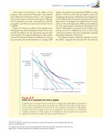
The higher of the two curves in Figure 14.1 represents the MRPL curve for a
firm in a competitive output market. Note that because there are diminishing
marginal returns to labor, the marginal product of labor falls as the amount of
labor increases. The marginal revenue product curve thus slopes downward,
even though the price of the output is constant.
1

We implicitly assume that all inputs to production are identical in quality. Differences in workers’
skills and abilities are discussed in Chapter 17.