(8th edition) (the pearson series in economics) robert pindyck, daniel rubinfeld microecon 270

CHAPTER 7 • The Cost of Production 245

with sunk costs. Rather, we can now focus on how a firm takes these prices into
account when determining how much capital and labor to utilize.7

The Isocost Line
We begin by looking at the cost of hiring factor inputs, which can be represented
by a firm’s isocost lines. An isocost line shows all possible combinations of labor
and capital that can be purchased for a given total cost. To see what an isocost
line looks like, recall that the total cost C of producing any particular output is
given by the sum of the firm’s labor cost wL and its capital cost rK:
C = wL + rK

(7.2)

For each different level of total cost, equation (7.2) describes a different isocost
line. In Figure 7.3, for example, the isocost line C0 describes all possible combinations of labor and capital that cost a total of C0 to hire.
If we rewrite the total cost equation as an equation for a straight line, we get
K = C/r - (w/r)L
It follows that the isocost line has a slope of ⌬K/⌬L ϭ −(w/r), which is the ratio of
the wage rate to the rental cost of capital. Note that this slope is similar to the slope
of the budget line that the consumer faces (because it is determined solely by the
prices of the goods in question, whether inputs or outputs). It tells us that if the firm
gave up a unit of labor (and recovered w dollars in cost) to buy w/r units of capital
at a cost of r dollars per unit, its total cost of production would remain the same. For
example, if the wage rate were $10 and the rental cost of capital $5, the firm could
replace one unit of labor with two units of capital with no change in total cost.

Choosing Inputs
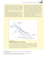
Suppose we wish to produce at an output level q1. How can we do so at minimum
cost? Look at the firm’s production isoquant, labeled q1, in Figure 7.3. The problem

is to choose the point on this isoquant that minimizes total cost.
Figure 7.3 illustrates the solution to this problem. Suppose the firm were to
spend C0 on inputs. Unfortunately, no combination of inputs can be purchased
for expenditure C0 that will allow the firm to achieve output q1. However, output
q1 can be achieved with the expenditure of C2, either by using K2 units of capital
and L2 units of labor, or by using K3 units of capital and L3 units of labor. But C2
is not the minimum cost. The same output q1 can be produced more cheaply, at a
cost of C1, by using K1 units of capital and L1 units of labor. In fact, isocost line C1 is
the lowest isocost line that allows output q1 to be produced. The point of tangency
of the isoquant q1 and the isocost line C1 at point A gives us the cost-minimizing
choice of inputs, L1 and K1, which can be read directly from the diagram. At this
point, the slopes of the isoquant and the isocost line are just equal.
When the expenditure on all inputs increases, the slope of the isocost line does
not change because the prices of the inputs have not changed. The intercept, however, increases. Suppose that the price of one of the inputs, such as labor, were
to increase. In that case, the slope of the isocost line −(w/r) would increase in

7

It is possible, of course, that input prices might increase with demand because of overtime or a relative shortage of capital equipment. We discuss the possibility of a relationship between the price of
factor inputs and the quantities demanded by a firm in Chapter 14.

• isocost line Graph showing
all possible combinations of
labor and capital that can be
purchased for a given total cost.