(8th edition) (the pearson series in economics) robert pindyck, daniel rubinfeld microecon 274

CHAPTER 7 • The Cost of Production 249

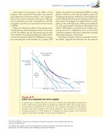
When the effluent fee is imposed, the cost of wastewater increases from $10 per gallon to $20: For every
gallon of wastewater (which costs $10), the firm has to
pay the government an additional $10. The effluent
fee therefore increases the cost of wastewater relative
to capital. To produce the same output at the lowest
possible cost, the manager must choose the isocost
line with a slope of −$20/$40 = −0.5 that is tangent to
the isoquant. In Figure 7.5, DE is the appropriate isocost line, and B gives the appropriate combination of
capital and wastewater. The move from A to B shows
that with an effluent fee the use of an alternative production technology that emphasizes the greater use
of capital (3500 machine-hours) and less production
of wastewater (5000 gallons) is cheaper than the

original process, which did not emphasize recycling.
Note that the total cost of production has increased
to $240,000: $140,000 for capital, $50,000 for wastewater, and $50,000 for the effluent fee.
We can learn two lessons from this decision.
First, the more easily factors can be substituted in
the production process—that is, the more easily
the firm can deal with its taconite particles without
using the river for waste treatment—the more effective the fee will be in reducing effluent. Second, the
greater the degree of substitution, the less the firm
will have to pay. In our example, the fee would have
been $100,000 had the firm not changed its inputs.
By moving production from A to B, however, the
steel company pays only a $50,000 fee.

Cost Minimization with Varying Output Levels
In the previous section we saw how a cost-minimizing firm selects a combination of inputs to produce a given level of output. Now we extend this analysis to

see how the firm’s costs depend on its output level. To do this, we determine the
firm’s cost-minimizing input quantities for each output level and then calculate
the resulting cost.
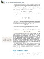
The cost-minimization exercise yields the result illustrated by Figure 7.6. We
have assumed that the firm can hire labor L at w = $10/hour and rent a unit of
capital K for r = $20/hour. Given these input costs, we have drawn three of the
firm’s isocost lines. Each isocost line is given by the following equation:
C = ($10/hour)(L) + ($20/hour)(K)
In Figure 7.6 (a), the lowest (unlabeled) line represents a cost of $1000, the middle
line $2000, and the highest line $3000.
You can see that each of the points A, B, and C in Figure 7.6 (a) is a point of
tangency between an isocost curve and an isoquant. Point B, for example, shows
us that the lowest-cost way to produce 200 units of output is to use 100 units
of labor and 50 units of capital; this combination lies on the $2000 isocost line.
Similarly, the lowest-cost way to produce 100 units of output (the lowest unlabeled isoquant) is $1000 (at point A, L = 50, K = 25); the least-cost means of
getting 300 units of output is $3000 (at point C, L = 150, K = 75).
The curve passing through the points of tangency between the firm’s isocost
lines and its isoquants is its expansion path. The expansion path describes the
combinations of labor and capital that the firm will choose to minimize costs
at each output level. As long as the use of both labor and capital increases with
output, the curve will be upward sloping. In this particular case we can easily
calculate the slope of the line. As output increases from 100 to 200 units, capital
increases from 25 to 50 units, while labor increases from 50 to 100 units. For each
level of output, the firm uses half as much capital as labor. Therefore, the expansion path is a straight line with a slope equal to
⌬K/⌬L = (50 - 25)/(100 - 50) =

1
2

• expansion path Curve

passing through points of
tangency between a firm’s
isocost lines and its isoquants.