(8th edition) (the pearson series in economics) robert pindyck, daniel rubinfeld microecon 137

112 PART 2 • Producers, Consumers, and Competitive Markets
demands of other people. These effects play a crucial role in the demands
for many high-tech products, such as computer hardware and software,
and telecommunications systems.
6. Finally, we will briefly describe some of the methods that economists use
to obtain empirical information about demand.

4.1 Individual Demand
This section shows how the demand curve of an individual consumer follows
from the consumption choices that a person makes when faced with a budget
constraint. To illustrate these concepts graphically, we will limit the available goods to food and clothing, and we will rely on the utility-maximization
approach described in Section 3.3 (page 86).

Price Changes
In §3.3, we explain how
a consumer chooses the
market basket on the highest indifference curve that
touches the consumer’s
budget line.

In §3.2, we explain how
the budget line shifts in
response to a price change.

• price-consumption
curve Curve tracing the utilitymaximizing combinations of
two goods as the price of one
changes.

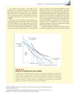
We begin by examining ways in which the consumption of food and clothing changes when the price of food changes. Figure 4.1 shows the consumption choices that a person will make when allocating a fixed amount of income
between the two goods.

Initially, the price of food is $1, the price of clothing $2, and the consumer’s income $20. The utility-maximizing consumption choice is at point B in
Figure 4.1 (a). Here, the consumer buys 12 units of food and 4 units of clothing,
thus achieving the level of utility associated with indifference curve U2.
Now look at Figure 4.1 (b), which shows the relationship between the price of
food and the quantity demanded. The horizontal axis measures the quantity of
food consumed, as in Figure 4.1 (a), but the vertical axis now measures the price
of food. Point G in Figure 4.1 (b) corresponds to point B in Figure 4.1 (a). At G,
the price of food is $1, and the consumer purchases 12 units of food.
Suppose the price of food increases to $2. As we saw in Chapter 3, the budget
line in Figure 4.1 (a) rotates inward about the vertical intercept, becoming twice
as steep as before. The higher relative price of food has increased the magnitude
of the slope of the budget line. The consumer now achieves maximum utility
at A, which is found on a lower indifference curve, U1. Because the price of food
has risen, the consumer’s purchasing power—and thus attainable utility—has
fallen. At A, the consumer chooses 4 units of food and 6 units of clothing. In
Figure 4.1 (b), this modified consumption choice is at E, which shows that at a
price of $2, 4 units of food are demanded.
Finally, what will happen if the price of food decreases to 50 cents? Because the
budget line now rotates outward, the consumer can achieve the higher level of
utility associated with indifference curve U3 in Figure 4.1 (a) by selecting D, with
20 units of food and 5 units of clothing. Point H in Figure 4.1 (b) shows the price
of 50 cents and the quantity demanded of 20 units of food.

The Individual Demand Curve
We can go on to include all possible changes in the price of food. In Figure 4.1 (a),
the price-consumption curve traces the utility-maximizing combinations of
food and clothing associated with every possible price of food. Note that as the
price of food falls, attainable utility increases and the consumer buys more food.
This pattern of increasing consumption of a good in response to a decrease in