(8th edition) (the pearson series in economics) robert pindyck, daniel rubinfeld microecon 139

114 PART 2 ã Producers, Consumers, and Competitive Markets
In Đ3.1, we introduce the
marginal rate of substitution
(MRS) as a measure of the
maximum amount of one
good that the consumer is
willing to give up in order to
obtain one unit of another
good.

2. At every point on the demand curve, the consumer is maximizing utility by
satisfying the condition that the marginal rate of substitution (MRS) of food
for clothing equals the ratio of the prices of food and clothing. As the price of
food falls, the price ratio and the MRS also fall. In Figure 4.1 (b), the price ratio
falls from 1 ($2/$2) at E (because the curve U1 is tangent to a budget line with
a slope of -1 at A) to 1/2 ($1/$2) at G, to 1/4 ($0.50/$2) at H. Because the consumer is maximizing utility, the MRS of food for clothing decreases as we move
down the demand curve. This phenomenon makes intuitive sense because it
tells us that the relative value of food falls as the consumer buys more of it.
The fact that the MRS varies along the individual’s demand curve tells us
something about how consumers value the consumption of a good or service.
Suppose we were to ask a consumer how much she would be willing to pay
for an additional unit of food when she is currently consuming 4 units. Point
E on the demand curve in Figure 4.1 (b) provides the answer: $2. Why? As we
pointed out above, because the MRS of food for clothing is 1 at E, one additional
unit of food is worth one additional unit of clothing. But a unit of clothing costs
$2, which is, therefore, the value (or marginal benefit) obtained by consuming
an additional unit of food. Thus, as we move down the demand curve in Figure
4.1 (b), the MRS falls. Likewise, the value that the consumer places on an additional unit of food falls from $2 to $1 to $0.50.

Income Changes

• income-consumption
curve Curve tracing the utilitymaximizing combinations of two
goods as a consumer’s income
changes.

We have seen what happens to the consumption of food and clothing when the
price of food changes. Now let’s see what happens when income changes.
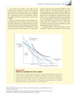
The effects of a change in income can be analyzed in much the same way as a
price change. Figure 4.2 (a) shows the consumption choices that a consumer will
make when allocating a fixed income to food and clothing when the price of food
is $1 and the price of clothing $2. As in Figure 4.1 (a), the quantity of clothing is
measured on the vertical axis and the quantity of food on the horizontal axis.
Income changes appear as changes in the budget line in Figure 4.2 (a). Initially,
the consumer’s income is $10. The utility-maximizing consumption choice is
then at A, at which point she buys 4 units of food and 3 units of clothing.
This choice of 4 units of food is also shown in Figure 4.2 (b) as E on demand
curve D1. Demand curve D1 is the curve that would be traced out if we held
income fixed at $10 but varied the price of food. Because we are holding the price
of food constant, we will observe only a single point E on this demand curve.
What happens if the consumer’s income is increased to $20? Her budget line
then shifts outward parallel to the original budget line, allowing her to attain
the utility level associated with indifference curve U2. Her optimal consumption choice is now at B, where she buys 10 units of food and 5 units of clothing.
In Figure 4.2 (b) her consumption of food is shown as G on demand curve D2.
D2 is the demand curve that would be traced out if we held income fixed at $20
but varied the price of food. Finally, note that if her income increases to $30,
she chooses D, with a market basket containing 16 units of food (and 7 units of
clothing), represented by H in Figure 4.2 (b).
We could go on to include all possible changes in income. In Figure 4.2 (a),
the income-consumption curve traces out the utility-maximizing combinations of food and clothing associated with every income level. The incomeconsumption curve in Figure 4.2 slopes upward because the consumption of both food and clothing increases as income increases. Previously, we
saw that a change in the price of a good corresponds to a movement along a

demand curve. Here, the situation is different. Because each demand curve is