Báo cáo khoa học: Kinetics of intra- and intermolecular zymogen activation with formation of an enzyme–zymogen complex ppt
Bạn đang xem bản rút gọn của tài liệu. Xem và tải ngay bản đầy đủ của tài liệu tại đây (222.04 KB, 12 trang )
Kinetics of intra- and intermolecular zymogen activation
with formation of an enzyme–zymogen complex
Matilde Esther Fuentes, Ramo
´
n Varo
´
n, Manuela Garcı
´a-Moreno
and Edelmira Valero
Grupo de Modelizacio
´
n en Bioquı
´
mica, Departamento de Quı
´
mica-Fı
´
sica, Escuela Polite
´
cnica Superior de Albacete, Universidad de Castilla-La
Mancha, Albacete, Spain
Living organisms possess different systems of biologi-
cal amplification that help them achieve a fast response
to a given stimulus in substrate cycling [1–3], enzyme
cascades [4,5] and limited proteolysis reactions [6–9].
Limited proteolysis is an irreversible and exergonic
reaction under normal physiological conditions, and
there is no opposite reaction that regenerates the same
hydrolyzed peptidic bond or that reinserts the corres-
ponding released peptide. Proenzyme activation there-
fore is a control mechanism that differs essentially
from allosteric transitions and reversible covalent modi-
fications.
Proenzyme activation by proteolytic cleavage of one
or more peptide bonds requires the presence of an acti-
vating enzyme. In those cases in which the activating
enzyme is the same as the activated one, the proenzyme
activation process is termed autocatalytic. Physiological
examples include the activation of trypsinogen into
trypsin [10,11], the conversion of pepsinogen into pep-
sin [12–14], and prekallikrein into kallikrein [15,16].
Several reports describe the kinetic behaviour of
enzyme systems involving autocatalytic zymogen activa-
tion – with or without steps in rapid equilibrium condi-
tions – in the presence [17] and absence [18] of a
substrate of the enzyme to monitor the reaction through
the release of product, and also in the presence of an
inhibitor of the enzyme [19,20]. In all of these contribu-
tions, the zymogen was considered to be without enzyme
activity. Nevertheless, references to the enzyme activity
of zymogens are increasingly more frequent [21–23].
Keywords
autocatalysis; enzyme kinetics; pepsin;
pepsinogen; zymogen
Correspondence
E. Valero, Grupo de Modelizacio
´
nen
Bioquı
´
mica, Departamento de Quı
´
mica-
Fı
´
sica, Escuela Polite
´
cnica Superior de
Albacete, Universidad de Castilla-La
Mancha, Avda. Espan˜a s⁄ n, Campus
Universitario, E-02071 Albacete, Spain
Fax: +34 967 59 92 24
Tel: +34 967 59 92 00
E-mail:
Note
The mathematical model described here has
been submitted to the Online Cellular
Systems Modelling Database and can be
accessed free of charge at: http://
jjj.biochem.sun.ac.za/database/fuentes/
index.html
(Received 6 July 2004, revised 6 September
2004, accepted 9 September 2004)
doi:10.1111/j.1432-1033.2004.04400.x
A mathematical description was made of an autocatalytic zymogen activa-
tion mechanism involving both intra- and intermolecular routes. The
reversible formation of an active intermediary enzyme–zymogen complex
was included in the intermolecular activation route, thus allowing a Micha-
elis–Menten constant to be defined for the activation of the zymogen
towards the active enzyme. Time–concentration equations describing the
evolution of the species involved in the system were obtained. In addition,
we have derived the corresponding kinetic equations for particular cases of
the general model studied. Experimental design and kinetic data analysis
procedures to evaluate the kinetic parameters, based on the derived kinetic
equations, are suggested. The validity of the results obtained were checked
by using simulated progress curves of the species involved. The model is
generally good enough to be applied to the experimental kinetic study of
the activation of different zymogens of physiological interest. The system
is illustrated by following the transformation kinetics of pepsinogen into
pepsin.
FEBS Journal 272 (2005) 85–96 ª 2004 FEBS 85
Al-Janabi et al. (1972) [12] offered kinetic evidence
for the existence of two activation pathways (intra-
and intermolecular) for the activation of pepsinogen to
pepsin, as is indicated in Scheme 1. They also obtained
the concentration–time kinetic equation for the pepsi-
nogen concentration, valid for the whole course of the
reaction and which was still used in recent contribu-
tions [23]. Subsequently, a number of different mecha-
nisms for the activation process of pepsinogen were
proposed by Koga and Hayashi (1976) [24]. By com-
paring the simulated progress curves obtained for each
of these mechanisms with the experimental results,
these authors suggested a reaction mechanism inclu-
ding both intra- and intermolecular activation of
the zymogen by the action of the active enzyme
(Scheme 2). This mechanism takes into account the
(irreversible) formation of a dimeric intermediate.
However, in the above contribution, no analytical
approximate solutions of the suggested mechanism
were obtained.
Taking into account the reaction in Schemes 1 and 2
concerning pepsinogen activation, we suggest a general
mechanism (Scheme 3) applicable to any zymogen acti-
vation, for which we have carried out a kinetic ana-
lysis. The above mechanism exhibits simultaneously two
catalytic routes, an intramolecular activation process,
route a, and an autocatalytic zymogen activation pro-
cess catalyzed by the same enzyme it produces, route
b. This mechanism includes the reversible formation of
an intermediary active enzyme–zymogen complex in
the intermolecular activation step. Both routes interact
because route a diminishes zymogen concentration,
increasing the active enzyme concentration, and there-
fore influences route b. In turn, route b also decreases
zymogen concentration, having an effect on route a.
Nevertheless, as we will see below, there are some
experimental conditions in which it can be assumed
that route b does not influence route a (but not vice
versa), so that the latter can be analysed independ-
ently. This mechanism is general enough to be applied
to different zymogens exhibiting both intra- and inter-
molecular reactions including, as particular cases,
those which reach rapid equilibrium (Scheme 4) and
the simplest reaction showing the two mentioned
routes in the absence of an EZ complex (Scheme 5).
Scheme 1. Mechanism for the autoactivation of pepsinogen to
pepsin [12]. Pgn, pepsinogen; Pep, pepsin.
Scheme 2. Mechanism suggested by Koga and Hayashi [24] invol-
ving two pH-dependent steps and a nonlinear reaction containing a
looped reaction with a dimeric intermediate, in which the peptide
fragments are released and pepsinogen is converted to pepsin. X
1
and X
2
are the unprotonated and protonated pepsinogen, respect-
ively, while X
3
*andX
4
* are structural isomers of the active pepsin
which are in an equilibrium involving proton binding. X
5
is the
dimeric intermediate.
Scheme 3. General mechanism proposed for the autoactivation of
zymogens involving both the intra (route a) and intermolecular
(route b) steps. Z is the zymogen, E is both the activating protease
and the activated enzyme, EZ is the complex enzyme–substrate
intermediate of the reaction, and W is one or more peptides
released from Z during the formation of E.
Scheme 4. Mechanism shown in Scheme 3 under rapid equilibrium
conditions between E, Z and EZ.
Scheme 5. Simplified general mechanism for the autoactivation of
zymogens.
Autocatalytic zymogen activation M. E. Fuentes et al.
86 FEBS Journal 272 (2005) 85–96 ª 2004 FEBS
Note that in Scheme 3, (Z) includes both X
1
and X
2
from Scheme 2 and (E) includes both X
3
* and X
4
*, so
that [Z] ¼ [X
1
]+[X
2
] and [E] ¼ [X
3
*] + [X
4
*]. Also,
note that Scheme 5 corresponds to Scheme 1 (previ-
ously reported by Al-Janabi et al. [12]), when Z and E
denote Pgn and Pep, respectively.
The aims of the present paper are: (a) to analyse the
complete kinetics for Scheme 3, obtaining approximate
analytical solutions and to confirm their goodness by
numerical simulation; (b) from the above results, to
derive other approximate solutions for Scheme 3 in sim-
plified conditions that arise from certain relations
between the values of the first or pseudo first-order rate
constants; (c) to derive the kinetic equations correspond-
ing to Schemes 4 and 5 – which can be considered par-
ticular cases of Scheme 3 when certain relations between
the values of the first or pseudo first-order rate constants
are observed – and (d) from the equations derived in (b),
to suggest an experimental design and a kinetic data
analysis to evaluate the kinetic parameters involved in
Scheme 3, which is immediately applicable to Schemes 4
and 5. All of these results are illustrated by the kinetics
of the autoactivation of pepsinogen to pepsin.
The mathematical model described here has been
submitted to the Online Cellular Systems Modelling
Database and can be accessed at: chem.
sun.ac.za/database/fuentes/index.html free of charge.
Theory
Notation and definitions
[E], [Z], [EZ], [W]: instantaneous concentrations of the
species E, Z, EZ and W, respectively. [E]
0
,[Z]
0
,[EZ]
0
,
[W]
0
: initial concentrations of the species E, Z, EZ and
W, respectively.
The dissociation constant of the EZ complex will be:
K
2
¼
k
2
k
2
The presence of EZ complex allows the definition of a
Michaelis–Menten constant for the activation of zymo-
gen towards its active enzyme as follows:
K
m
¼
k
2
þ k
3
k
2
Time course differential equations and mass
balances
The kinetic behaviour of the species E, Z, EZ and W
involved in Scheme 3 is described by the following set
of differential equations (Eqns 1–4):
d½ Z
dt
¼k
1
½Zk
2
½Z½Eþk
2
½EZð1Þ
d½E
dt
¼ k
1
½Zk
2
½Z½Eþðk
2
þ 2k
3
Þ½EZð2Þ
d½ EZ
dt
¼ k
2
½Z½Eðk
2
þ k
3
Þ½EZð3Þ
d½W
dt
¼ k
1
½Zþk
3
½EZð4Þ
This set of differential equations is nonlinear and, in
order to obtain analytical solutions, we shall assume
that the concentration of Z remains approximately
constant during the course of the reaction (Eqn 5), i.e.
½Z½Z
0
ð5Þ
Taking into account this assumption, the differential
equation system that describes the mechanism shown
in Scheme 3 is given by Eqns (6–8):
d½ E
dt
¼ k
1
½Z
0
k
2
½Z
0
½Eþðk
2
þ 2k
3
Þ½EZð6Þ
d½EZ
dt
¼ k
2
½Z
0
½Eðk
2
þ k
3
Þ½EZð7Þ
d½ W
dt
¼ k
1
½Z
0
þ k
3
½EZð8Þ
The differential Eqns (6) and (7) constitute a nonho-
mogeneous linear system that may become homogen-
eous by further derivation and by performing the
changes in the variables d[E] ⁄ dt ¼ X, and d [EZ] ⁄ dt ¼
Y, giving Eqns (9) and (10):
dX
dt
¼k
2
½Z
0
X þðk
2
þ 2k
3
ÞY ð9Þ
dY
dt
¼ k
2
½Z
0
X ðk
2
þ k
3
ÞY ð10Þ
the initial conditions of which are at t ¼ 0, X ¼
k
1
[Z]
0
, and Y ¼ 0, taking into account that [E]
0
¼ 0
and [EZ]
0
¼ 0. The solution to this system is given by
Eqns (11) and (12):
X ¼
k
1
½Z
0
ðk
2
½Z
0
þ k
2
Þ
k
1
k
2
e
k
1
t
þ
k
1
½Z
0
ðk
2
½Z
0
þ k
1
Þ
k
1
k
2
e
k
2
t
ð11Þ
Y ¼
k
1
k
2
½Z
2
0
k
1
k
2
ðe
k
1
t
e
k
2
t
Þð12Þ
where:
M. E. Fuentes et al. Autocatalytic zymogen activation
FEBS Journal 272 (2005) 85–96 ª 2004 FEBS 87
k
1
¼
ðk
2
½Z
0
þk
2
þk
3
Þþ
ffiffiffiffiffiffiffiffiffiffiffiffiffiffiffiffiffiffiffiffiffiffiffiffiffiffiffiffiffiffiffiffiffiffiffiffiffiffiffiffiffiffiffiffiffiffiffiffiffiffiffiffiffiffiffiffiffiffiffi
ðk
2
½Z
0
þk
2
þk
3
Þ
2
þ4k
2
k
3
½Z
0
q
2
ð13Þ
k
2
¼
ðk
2
½Z
0
þk
2
þk
3
Þ
ffiffiffiffiffiffiffiffiffiffiffiffiffiffiffiffiffiffiffiffiffiffiffiffiffiffiffiffiffiffiffiffiffiffiffiffiffiffiffiffiffiffiffiffiffiffiffiffiffiffiffiffiffiffiffiffiffiffiffi
ðk
2
½Z
0
þk
2
þk
3
Þ
2
þ4k
2
k
3
½Z
0
q
2
ð14Þ
Note that both k
1
and k
2
are real quantities, k
1
always
being positive and k
2
negative, and that the relations
between k
1
and k
2
are as follow (Eqns 15–17):
k
1
þ k
2
¼ðk
2
½Z
0
þ k
2
þ k
3
Þð15Þ
k
1
k
2
¼k
2
k
3
½Z
0
ð16Þ
k
1
< jk
2
jð17Þ
To return to our original symbolism, Eqns (11) and
(12) are integrated and, taking into account the initial
conditions mentioned above, gives:
½E¼A
1;0
þ A
1;1
e
k
1
t
þ A
1;2
e
k
2
t
ð18Þ
½EZ¼A
2;0
þ A
2;1
e
k
1
t
þ A
2;2
e
k
2
t
ð19Þ
The expressions corresponding to A
i,j
(i ¼ 1, 2, 3, 4;
j ¼ 0, 1, 2) are given in the Appendix A (Eqns
A1–A12).
If the progress of the reaction is followed by
measuring the instantaneous zymogen concentration,
the following mass balance must be taken into
account:
½Z¼½Z
0
½E2½EZð20Þ
Inserting Eqns (18) and (19) into Eqn (20), the follow-
ing time-concentration equation (Eqn 21) is obtained:
½Z¼A
3;0
þ A
3;1
e
k
1
t
þ A
3;2
e
k
2
t
ð21Þ
This equation could also be obtained by integration of
Eqn (1) after inserting into it condition 5 (Eqn 5) and
Eqns (18) and (19).
To obtain the equation describing the accumulation
of the peptide product of catalysis, Eqn (19) is inserted
into Eqn (8) and, by integrating again, and taking into
account the initial condition [W]
0
¼ 0, we obtain Eqn
(22):
½W ¼A
4;0
þ A
4;1
e
k
1
t
þ A
4;2
e
k
2
t
ð22Þ
This equation could also be obtained from Eqns (19)
and (21), taking into account the following mass bal-
ance:
½W ¼½Z
0
½Z½EZð23Þ
Equation (21) for zymogen consumption is different
from the equation reported previously in the literature
for the simplified reaction mechanism shown in
Scheme 1 [12]. To obtain this latter equation, the reac-
tion mechanism was simplified, disregarding the inter-
mediary zymogen-active enzyme complex, as this is the
only way to obtain a concentration–time relation for
the whole course of the reaction, but which clearly cor-
responds to a reaction mechanism which does not take
into account reality. The equations derived here have
the advantage that they respond to a mechanism close
to that which occurs in reality, including the formation
of an EZ complex in the intermolecular activation
step. However, they have the disadvantage of being
only valid for a relatively short time, with the corres-
ponding experimental difficulties. The measurement of
zymogen concentrations not far from the initial value
in a short-time reaction leads to unavoidable experi-
mental errors. Nevertheless, taking into account that
the values of the kinetic parameters are independent of
the reaction time registered, this will allow the evalua-
tion of kinetic parameters involved in the system
whenever the reaction can experimentally be followed.
Once the value of the kinetic parameters are obtained,
the behaviour of the reaction can be predicted until
the zymogen is exhausted.
Results and Discussion
We obtained the time course equations for the species
involved in the reaction corresponding to the autocata-
lytic activation of a zymogen, including the formation
of an active enzyme–zymogen complex (Scheme 3).
The reaction scheme suggested is the most simple one
that covers the main features described in the litera-
ture, i.e. a route of intramolecular activation of the
zymogen into the active enzyme, E, and one or more
peptides represented by W [route (a), Scheme 3]
[12,22,25–27] and a route of autocatalytic activation of
zymogen by the active enzyme formed (route (b),
Scheme 3, [12,26,28]).
Route (a) of Scheme 3 condenses, in a single step,
the whole process corresponding to a conformational
change of Z molecules brought about by low pH and
the subsequent cleavage of the N-terminal peptide [14].
Thus, k
1
is actually an apparent rate constant corres-
ponding to the whole process leading from Z to E and
W by intramolecular activation. Route (b) of Scheme 3
has been assumed to follow a single Michaelis–Menten
mechanism instead of the more general Uni–Bi mech-
anism. This approach is the usual one used to describe
Autocatalytic zymogen activation M. E. Fuentes et al.
88 FEBS Journal 272 (2005) 85–96 ª 2004 FEBS
mechanisms of autocatalytic zymogen activation and
has been sufficiently justified [11,29–31].
Previously, kinetic analyses of the reactions, whereby
a zymogen is activated both intra- and intermole-
cularly by the action of the active enzyme, have been
made and used for the experimental determination of
the kinetic parameters involved in pepsinogen autoacti-
vation [12,21,23,32]. However these contributions used
the simplified reaction mechanism shown in Scheme 5
(which coincides with Scheme 1), i.e. the equilibrium
between the species E, Z and EZ in the intermolecular
activation step was not taken into account. It is this
step that we include in the present paper, with the
additional advantage that the results obtained using
this novel approach are nearer reality [24,26]. For
greater clarity and to better imitate the physiological
conditions, we assumed in our analysis that no active
enzyme is present at the onset of the reaction, but only
the zymogen.
Validity of the time course equations derived
Kinetic equations for all the species involved in
Scheme 3 were derived by solving the nonhomogene-
ous set of ordinary, linear (with constant coefficients),
differential Eqns (6–8). These kinetic equations are
valid whenever condition 5 (Eqn 5) holds, and for this
reason they are approximate analytical solutions. They
can be further simplified in such a way that a kinetic
analysis of the experimental kinetic data make it pos-
sible to completely characterize the system. Obviously,
the approximate analytical time course equations
derived here are also applicable to any zymogen acti-
vation mechanism described by Scheme 3 in the same
initial and experimental conditions.
As [Z] continuously decreases from the beginning of
the reaction, the longer the reaction time, the less accu-
rate the analytical solutions. This is usual in enzyme
kinetics, where to derive approximate analytical solu-
tions corresponding either to the transient phase or the
steady-state of an enzymatic reaction, substrate con-
centration (the zymogen in this case) is usually
assumed to remain approximately constant [33–35] and
therefore the results obtained are only valid under this
condition. It is obvious that if the reaction is allowed
to progress, the final concentration of zymogen will be
zero. Thus, as is common practice in assays on enzyme
kinetics, the reaction can only be allowed to evolve to
a small extent during the assays compared with the
total reaction time taken for the substrate to vanish
[36]. Obviously, the more the zymogen concentration
diminishes, the less accurate the equations obtained
become.
Experimentally, it is possible to determine whether
the assumption 5 (Eqn 5), which is always true at the
onset of the reaction, is still fulfilled at a certain reac-
tion time. The fraction, q, of the remaining zymogen is
introduced as:
q ¼
½Z
½Z
0
ð24Þ
and we may arbitrarily set the q-value (e.g. q ¼ 0.7)
above which the approximate solutions remains applic-
able. Thus, the [Z]-values for which the equations
obtained are applicable are:
½Zq½Z
0
ð25Þ
For example, if [Z]
0
¼ 10
)3
m and q ¼ 0.7, then,
according to Eqn (25), the analytical equations derived
here will be valid only when [Z] ‡ 7 · 10
)4
m.
To illustrate the degree of validity of our approach,
in Fig. 1A we show the time progress curves obtained
by numerical integration of the entire differential equa-
tion system obtained directly from the mechanism
shown in Scheme 3 (Eqns 1–4), for an arbitrary set of
rate constants values and [Z]
0
-value. A comparison of
the results obtained above for [Z] with those obtained
from the equation derived here Eqn (21) and from the
equation previously reported in the literature for
Scheme 1 (Eqn B1, Appendix B) [12] is shown in
Fig. 1B, using the same values for the rate constants
and initial conditions. Table 1 shows a numerical com-
parison of these data for different q-values, including
the relative errors of the [Z] values predicted by the
two integrated equations with respect to those
obtained from the numerical solution at the same
times. As can be seen, as long as q remains higher than
0.7, the relative error committed using the equations
derived here remain below 10%, nevertheless it is
greater when the EZ complex is not taken into
account.
Uni-exponential kinetic behaviour
The time course equations here obtained are of the
bi-exponential type. Nevertheless, because k
1
is positive
and k
2
negative, and due to the relationship in Eqn
(17), the negative exponential term in Eqn (21) can be
neglected from a relative short time after the onset of
the reaction, so that the kinetic behaviour of all of the
species becomes uni-exponential from this time. The
higher the value of |k
2
| compared with k
1
, the shorter
the time from which the kinetic behaviour can be con-
sidered uni-exponential. In this way, the kinetic equa-
tions for Z (Eqn 26) and W (Eqn 27) become:
M. E. Fuentes et al. Autocatalytic zymogen activation
FEBS Journal 272 (2005) 85–96 ª 2004 FEBS 89
½Z¼A
3;0
þ A
3;1
e
k
1
t
ð26Þ
½W ¼A
4;0
þ A
4;1
e
k
1
t
ð27Þ
The case in which one exponential term can be
neglected after approximately t ¼ 0
In such a case, the following relations (Eqns 28–30)
must be fulfilled:
jk
2
jk
1
ð28Þ
i.e.
k
1
þ k
2
k
2
ð29Þ
k
1
k
2
k
2
ð30Þ
Under these conditions, the uni-exponential behaviour
of the species can be assumed from t ¼ 0. Thus, if the
relationships 29 and 30 [Eqns (29) and (30)] are inser-
ted into Eqns (26) and (27), we obtain:
½Z½Z
0
k
1
½Z
0
ðk
2
k
2
½Z
0
Þ
k
1
k
2
ðe
k
1
t
1Þðfrom t 0Þ
ð31Þ
½W
k
1
½Z
0
k
1
ðe
k
1
t
1Þðfrom t 0Þð32Þ
Bearing in mind the relation 29 (Eqn 29), Eqn (15)
becomes:
k
2
ðk
2
½Z
0
þ k
2
¼ k
3
Þð33Þ
and from Eqns (16) and (33) we obtain:
k
1
k
3
½Z
0
K
m
þ½Z
0
ð34Þ
The kinetic behaviour from the onset of the reaction is
a consequence of assumption 28 (Eqn 28). This condi-
tion is only fulfilled if certain relations between the
Fig. 1. (A) Simulated progress curves corresponding to the species
involved in the mechanism shown in Scheme 3. The values of the
rate constants used were: k
1
¼ 4.0 · 10
)3
Æs
)1
, k
2
¼ 1.0 · 10
3
M
)1
Æs
)1
, k
)2
¼ 2.1 · 10
)4
Æs
)1
and k
3
¼ 5.4 · 10
)4
Æs
)1
. The initial
zymogen concentration used was [Z]
0
¼ 2.4 · 10
)5
M. (B) Progress
curves corresponding to Z consumption obtained from numerical
integration (curve i), from Eqn (21) (curve ii) and from the equation
corresponding to the mechanism proposed by Al-Janabi et al. [12]
(Eqn B1), Appendix B (curve iii). Conditions as indicated in Fig. 1A.
Table 1. Values of [Z] obtained from the simulated curves ([Z]
sim
)
compared with those obtained from Eqn (21) ([Z]
Eqn 21
) and from
Eqn (B1) in Appendix B [12] ([Z]
Eqn B1
). The values of the rate con-
stants used were those indicated in Fig. 1 and the q-values corres-
pond to [Z]
sim
-values. In the third column we have indicated the
corresponding t-value at which the [Z]-values are reached. The fifth
and seventh columns correspond to the relative error of [Z]-values
obtained with Eqn (21) and Eqn (B1), respectively, compared with
[Z]
sim
-values.
q
(%)
[Z]
sim
(lM)
t
(s)
[Z]
Eqn 21
(lM)
Relative
error (%)
[Z]
Eqn B1
(lM)
Relative
error (%)
100 24.00 0.00 24.00 0.00 24.00 0.00
99 23.76 2.55 23.75 0.05 23.75 0.05
98 23.52 5.02 23.49 0.13 23.49 0.11
95 22.80 11.43 22.77 0.15 22.77 0.12
90 21.60 22.56 21.34 1.20 21.32 1.31
85 20.40 31.82 20.03 1.83 19.91 2.40
80 19.20 42.09 18.46 3.85 18.16 5.40
75 18.00 51.64 16.92 5.99 16.40 8.91
70 16.80 62.36 15.12 10.00 14.32 14.76
65 15.60 72.06 13.43 13.89 12.43 20.35
60 14.40 83.12 11.46 20.43 10.34 28.21
50 12.00 108.68 6.73 43.88 6.23 48.09
Autocatalytic zymogen activation M. E. Fuentes et al.
90 FEBS Journal 272 (2005) 85–96 ª 2004 FEBS
first- and pseudo first-order rate constants apply. We
have demonstrated that condition 28 (Eqn 28) leads to
Eqn (33) and therefore taking into account Eqn (14),
the following relationship is deduced:
ðk
2
½Z
0
þ k
2
þ k
3
Þ
2
4k
2
k
3
½Z
0
ð35Þ
i.e. condition 33 (Eqn 33) is a sufficient condition for
relationship 35 (Eqn 35) to exist. In turn, condition
28 (Eqn 28) is a sufficient condition for relationship
29 (Eqn 29). Indeed, if we insert condition 29 into
Eqn (15), k
2
is given by Eqn (33) and therefore
according to Eqn (14), relation 35 (Eqn 35) is
observed. Thus, conditions 28 (Eqn 28) and 35 (Eqn
35) are equivalent. This is expressed mathematically
as:
jk
2
jk
1
,ðk
2
½Z
0
þ k
2
þ k
3
Þ
2
4k
2
k
3
½Z
0
ð36Þ
That condition 35 (Eqn 35) is fulfilled, which justifies
the uni-exponential kinetic behaviour, is reasonable to
expect because k
3
is a rate constant corresponding to
the cleavage of a peptidic bond, i.e. to a covalent
modification, whereas k
-2
and k
2
[Z]
0
are rate con-
stants corresponding to the dissociation and forma-
tion of the EZ complex. It is therefore reasonable to
think that:
k
3
k
2
ð37Þ
and ⁄ or
k
3
k
2
½Z
0
ð38Þ
In both of the above cases condition 36 (Eqn 36) is
fulfilled. In the following we will denote, for greater
clarity, k
1
as k. Thus, we rewrite Eqns (31) and (34)
as:
½Z½Z
0
k
1
½Z
0
ðk
2
k
2
½Z
0
Þ
kk
2
ðe
kt
1Þð39Þ
k
k
3
Z½
0
K
m
þ Z½
0
ð40Þ
Rapid equilibrium assumptions: Scheme 4
A particular case of uni-exponential behaviour is that
corresponding to rapid equilibrium conditions, i.e. the
assumption that the reversible reaction step in
Scheme 3 is in equilibrium from the onset of the reac-
tion. For that, relations 37 and 38 (Eqns 37 and 38)
must be observed simultaneously. All equations for the
uni-exponential behaviour are applicable but, in this
case the Michaelis constant K
m
should be replaced in
Eqn (40) by the equilibrium constant K
2
:
k
k
3
½Z
0
K
2
þ½Z
0
ð41Þ
The case in which the activation can be
represented by Scheme 5
From a comparison of Schemes 3 and 5, it can be seen
that the latter formally arises from Scheme 3 if:
k
3
!1 ð42Þ
If we take into account condition 42 (Eqn 42), we see
that Eqn (36) is fulfilled and therefore uni-exponential
Eqns (39) and (40) are applicable, but now:
k k
2
½Z
0
ð43Þ
which is obtained as lim
k
3
!1
k; where k is given by
Eqn (40).
The case in which the intramolecular activation
of pepsinogen is predominant
In this case, the amount of zymogen activated inter-
molecularly by the active enzyme (route b) in Scheme
3 may be considered negligible and so it can be
assumed that:
k
2
0 ð44Þ
Therefore Eqn (33) is rewritten as:
k
2
¼ðk
2
þ k
3
Þð45Þ
Under these conditions, Eqn (39) can be rewritten as:
½Z½Z
0
k
1
½Z
0
k
ðe
kt
1Þð46Þ
which may be transformed into the uni-exponential
equation reported by Al-Janabi et al. [12] by substitu-
ting the exponential term by a series development, only
considering the two first terms for short reactions
times, and then returning to the exponential notation.
This gives:
½Z¼½Z
0
e
k
1
t
ð47Þ
Kinetic data analysis
The uni-exponential kinetic behaviour of the reaction
evolving according to Scheme 3 from the onset is the
most realistic because of condition [28] will probably
be fulfilled for the reasons given above. Thus, we will
confine ourselves to the general case of a uni-exponen-
tial behaviour given by Eqns (39–40). In this kinetic
analysis, it is assumed that the remaining zymogen,
M. E. Fuentes et al. Autocatalytic zymogen activation
FEBS Journal 272 (2005) 85–96 ª 2004 FEBS 91
[Z], can be experimentally monitored by a discontinu-
ous method [12,23].
The procedure we suggest is valid whenever
[E]+[EZ] remains much lower than [Z]
0
and consists
of the following two steps: (a) plotting the experimen-
tal [Z]-values obtained by any discontinuous method
at different reaction times, t, and at different [Z]
0
-val-
ues, and fitting them to Eqn (26), gives the correspond-
ing A
3,0
, A
3,1
, and k-values for the different initial
zymogen concentrations used; (b) Eqn (40) indicates
that the kinetic parameter k has a hyperbolic depend-
ence on initial zymogen concentration, [Z]
0
. Therefore,
the kinetic parameters k
3
and K
m
can be evaluated by
a nonlinear least-squares fit of the experimental k-val-
ues obtained in step (a) to this equation. Furthermore,
these parameters can also be obtained by linear regres-
sion by using any linearizing transformation of Eqn
(40), such as a Hanes–Woolf type plot ([Z]
0
⁄ k vs.
[Z]
0
). In this case, a straight-line will be obtained, with
the following properties:
ordinate intercept ¼
K
m
k
3
ð48Þ
slope ¼
1
k
3
ð49Þ
abscissa intercept ¼K
m
ð50Þ
Therefore, the kinetic parameters k
3
and K
m
can be
evaluated.
Particular cases of Scheme 3
Schemes 4 and 5 can be considered formally as partic-
ular cases of the reaction mechanism shown in
Scheme 3. The kinetic equations for these mechanisms
could be obtained from their corresponding system of
differential equations. However, they can also be
obtained faster and more easily from the differential
equations of the mechanism indicated in Scheme 3, by
converting it into the mechanism under study [37–39],
as has been done in the present paper.
Discrimination between Schemes 3, 4 and 5
The above described step (b) for evaluating the kinetic
parameters k
3
and K
m
involved in Eqns (39) and (40)
is also valid for evaluating the kinetic parameters
involved in Scheme 4 (Eqns 39 and 41) and Scheme 5
(Eqns 39 and 43), which are particular cases of
Scheme 3. It also serves to discriminate between them.
Thus, if the enzymatic system under study evolves
according to Scheme 4, in which case relations 37 and
38 (Eqns 37 and 38) are fulfilled, the K
m
value
obtained in step (b) of the above described procedure
will approximately coincide with K
2
, according to
Eqn (41). In turn, if the enzyme system evolves accord-
ing to Scheme 5, taking into account Eqns (39) and
(43), the intercept and the slope of the straight line ari-
sing from step (b) will become:
ordinate intercept ¼ lim
k
3
!1
ð
K
m
k
3
Þ¼
1
k
2
ð51Þ
slope ¼ lim
k
3
!1
ð
1
k
3
Þ¼0 ð52Þ
In this way, the suggested procedure for evaluating the
kinetic parameters allows us to discriminate between
Scheme 5 and Schemes 3 and 4. If the straight line ari-
sing from step (b) has a slope of zero or nearly zero,
then a compatible mechanism reaction is that des-
cribed by Scheme 5. If this is not the case, the mechan-
ism reaction is compatible with both Schemes 3 and 4,
between which it is impossible to discriminate. Never-
theless, because Scheme 4 corresponds to a situation in
which relations 37 and 38 (Eqns 37 and 38) are
observed, it is reasonable to think that the lower the
k
3
value, the more probable it is that the above men-
tioned relations will be observed. Thus, the higher the
ordinate intercept of the straight line arising from step
(b), the more probable the reaction scheme will be the
one described by Scheme 4 and that Eqn (41) is ful-
filled. To illustrate this, Eqn (40) is plotted in linear
form in Fig. 2 for fixed values of k
2
and k
-2
at different
k
3
values leading to Schemes 3, 4 and 5.
Pepsinogen autoactivation kinetics
The theoretical results obtained in the present paper
are illustrated by the kinetics of the activation of
pepsinogen to pepsin. Figure 3A shows the experimen-
tal progress curves corresponding to the remaining
pepsinogen in the reaction medium. The inset shows
the same results as percentage of remaining pepsino-
gen. Taking into account assumption 5 from the The-
ory section and the results shown in Table 1, the time
course of the reaction was followed in all cases until a
q-value of 0.7 was reached. These data were fitted by
nonlinear regression to Eqn (26), thus providing the
values of A
3,0
, A
3,1
and k at the different initial pepsi-
nogen concentrations used. Figure 3B shows these data
plotted according to the kinetic analysis here proposed.
Taking into account Eqns (48–50), the following values
for the kinetic parameters involved in the system were
obtained: k
3
¼ [6.13 ± 0.14] · 10
)4
Æs
)1
, K
m
¼ [1.50 ±
1.29], · 10
)7
m. This value of k
3
cannot be compared
with the value of the second order rate constant k
2
Autocatalytic zymogen activation M. E. Fuentes et al.
92 FEBS Journal 272 (2005) 85–96 ª 2004 FEBS
reported in the literature, as their corresponding units
are not the same [12]. In addition, because kinetic data
taking into consideration the formation of the EZ
complex have not been obtained before, the K
m
values
for the pepsinogen–pepsin system have not been repor-
ted either. Taking into account the discrimination
between Schemes 3, 4 and 5 proposed here and the
experimental results plotted in Fig. 3B, the reaction
mechanism is compatible with the formation of an EZ
complex, although it is not possible to discriminate
between Schemes 3 and 4.
It can be seen that the curves fitting the experimen-
tal data in Fig. 3A are approximately straight lines.
This fact can be explained by the following: the expo-
nential term in Eqn (39) can be substituted by a series
development, and taking into account that, for short
reaction times, only the two first terms may be consid-
ered significant, this equation is transformed into the
straight line equation:
½Z½Z
0
k
1
½Z
0
ð2k
2
½Z
0
þ k
2
þ k
3
Þ
k
2
½Z
0
þ k
2
þ k
3
t ð53Þ
whose ordinate intercept and slope are:
ordinate intercept ¼½Z
0
ð54Þ
slope ¼
k
1
½Z
0
ð2½Z
0
þ K
m
Þ
½Z
0
þ K
m
ð55Þ
From this equation it can be seen that the value of k
1
can be obtained from the slopes of plots of [Z] vs. time
at relatively short reaction times once K
m
is known,
giving the following value, k
1
¼ [5.14 ± 0.56] ·
10
)3
Æs
)1
. This value, which was obtained at 5 °C and
pH ¼ 2, together with the value obtained at 28 °C and
the same pH by Al-Janabi et al. [12] (k
1
Fig. 3. (A) Time course of pepsinogen consumption at different initial concentrations. Experimental conditions were as indicated in Experi-
mental procedures. The inset shows the same results as remaining pepsinogen (%). Lines have been shifted at five unit intervals for greater
clarity. The following initial concentrations of pepsinogen were used: (d) 1.52 · 10
)6
(s) 3.18 · 10
)6
(m) 4.84 · 10
)6
(n) 6.49 · 10
)6
and
(j) 8.17 · 10
)6
M. The points represent experimental data (they are the mean of three assays), the error bars represent SD, and the lines
correspond to data obtained by nonlinear regression analysis to Eqn (26). (B) Secondary plot of the above data as [Z]
0
⁄ k vs. [Z]
0
. k Values
were obtained by fitting experimental progress curves from Fig. 3A by nonlinear regression to Eqn (26), according to the kinetic analysis
here proposed. The points represent experimental data and the line corresponds to data obtained by linear regression analysis according to a
Hanes–Woolf rearrangement of Eqn (40).
Fig. 2. Plot of [Z]
0
⁄ k vs. [Z]
0
according to Eqn (40) for three differ-
ent k
3
values. Values of the rate constants k
2
and k
)2
were as indi-
cated in Fig. 1. The values used for k
3
were the following: curve i,
2 · 10
)2
s
)1
; curve ii,2· 10
)3
s
)1
and curve iii,2· 10
)4
s
)1
,
which correspond to Schemes 5, 3 and 4, respectively. The inset
shows an expansion of this graph near the coordinate origin.
M. E. Fuentes et al. Autocatalytic zymogen activation
FEBS Journal 272 (2005) 85–96 ª 2004 FEBS 93
4.33 · 10
)2
Æs
)1
) make it possible to estimate the values
of the preexponential factor, A, and the activation
energy, E
a
, involved in the Arrhenius equation [k
1
¼
A exp(–E
a
⁄ RT)], which provides the variation of the
rate constant, k
1
, corresponding to step (a) in Scheme 3.
The estimated values are A ¼ 6.75 · 10
9
s
)1
, E
a
¼
64.53 kJÆmol
)1
.
Furthermore, it can be observed from Fig. 3A that
the slopes of the plots obtained at different initial
zymogen concentrations tend to infinite when
[Z]
0
fi 1, and to zero when [Z]
0
fi 0, in agreement
with Eqn 55.
Concluding remarks
In conclusion, we have obtained new approximate
solutions for the kinetics of zymogen activation in con-
ditions where both intra- and intermolecular processes
take place. The proposed reaction scheme (Scheme 3)
is a modification of previous mechanisms for this kind
of processes [24], which were only treated by numerical
integration. The main innovation of the present paper
is that the kinetic behaviour of the system has been
analysed in both analytical and numerical ways, thus
showing the goodness of the analysis.
The above suggested mathematical analysis has been
applied to the pepsinogen–pepsin activation, which is
an interesting physiological enzymatic system.
Experimental procedures
Materials
Pepsinogen from porcine stomach (3300 unitsÆmg protein
)1
),
hemoglobin from bovine blood, pepstatin A, sodium citrate
and trichloroacetic acid were purchased from Sigma
(Madrid, Spain). Stock solutions of pepsinogen were pre-
pared daily by dissolving 6.5 mg of the zymogen in 5 mL of
0.02 m Tris ⁄ HCl buffer, pH 7.5. The hemoglobin solution
was also prepared daily by 4 : 1 dilution in 0.3 m HCl of a
stock solution of 2.5% (w ⁄ v) hemoglobin, filtered previously
through glass wool. The zymogen concentration was deter-
mined by active-site pepstatin A titration as a tight-binding
inhibitor [40]. All other buffers and reagents were of analyt-
ical grade and used without further purification. All solu-
tions were prepared in ultrapure deionized nonpyrogenic
water (Milli Q, Millipore Iberica, SA, Barcelona, Spain).
Methods
Assay for pepsinogen activation
The general scheme for these experiments was the same as
used earlier [12]. Aliquots of 100 lL of the stock solution
of pepsinogen were precooled at 5 °C. Then, 100 lLof
0.1 m sodium citrate ⁄ HCl buffer, pH 2.0, also at 5 °C, were
added to this solution, stirred, and after the appropiate
time intervals, 300 lL of 0.5 m Tris ⁄ HCl buffer, pH 8.5,
were added. These additions, by syringe, were made as
quickly as possible. The test tubes were introduced in a
water bath at 37 °C for 20 min, after which the solutions
were assayed for remaining pepsinogen activity. Solution
(100 lL) was now added to 1 mL of 0.2 m sodium cit-
rate ⁄ HCl buffer, pH 2.0, and allowed to activate for
20 min. Then, 1 mL hemoglobin solution was added to
each tube and, after exactly 10 min, 1 mL of 5% trichloro-
acetic acid solution was added. The mixture was filtered
through a poly(vinylidene difluoride) filter paper (pore
size ¼ 0.45 lm, diameter ¼ 13 mm) and the absorbance of
the filtrate was read at 280 nm against a blank containing
no enzyme. All the assays were performed in polypropylene
tubes [41]. Other activating pepsinogen concentrations were
assayed by appropriate dilution of the stock solution in
0.02 m Tris ⁄ HCl buffer, pH 7.5.
Assays at 5 °C were performed using a Hetofrig Selecta
bath with a heater ⁄ cooler using a commercial antifreeze
and checked using a Cole-Parmer digital thermometer with
a precision of ± 0.1 °C. A Precisterm Selecta water bath
was used for the experiments at 37 °C. Spectrophotometric
readings were obtained on a Uvikon 940 spectrophotometer
from Kontron Instruments, Zurich, Switzerland.
The experimental progress curves thus obtained were fit-
ted by nonlinear regression to Eqn 26 using the sigmaplot
scientific graphing system, version 8.02 (2002, SPSS Inc).
Numerical integration
Simulated progress curves were obtained by numerical
integration of the nonlinear set of differential equations
directly obtained from Scheme 3 (Eqns 1–4), using arbitrary
sets of rate constants and initial concentration values. This
numerical solution was found by the Runge–Kutta–Fehl-
berg algorithm [42,43] using a computer program imple-
mented in Visual C++ 6.0 [44]. The above program was
run on a PC compatible computer based on a Pentium
IV ⁄ 2 GHz processor with 512 Mb of RAM.
Acknowledgements
This work was supported by grants from the Comisio
´
n
Interministerial de Ciencia y Tecnologı
´
a (MCyT,
Spain), Project No. BQU2002-01960 and from Junta
de Comunidades de Castilla-La Mancha, Project No.
GC-02–032. M. E. F. has a fellowship from the Prog-
rama de Becas Predoctorales de Formacio
´
n de Perso-
nal Investigador (MCyT, Spain), associated to the
above Project, cofinanced by the European Social
Fund.
Autocatalytic zymogen activation M. E. Fuentes et al.
94 FEBS Journal 272 (2005) 85–96 ª 2004 FEBS
References
1 Newsholme EA, Challiss RAJ & Crabtree B (1984) Sub-
strate cycles: their role in improving sensitivity in meta-
bolic control. Trends in Biochem 9, 277–280.
2 Valero E, Varo
´
n R & Garcı
´
a-Carmona F (1995) Kinetic
study of an enzymic cycling system coupled to an enzy-
mic step: determination of alkaline phosphatase activity.
Biochem J 309, 181–185.
3 Valero E, Varo
´
n R & Garcı
´
a-Carmona F (1997) Mathe-
matical model for the determination of an enzyme activ-
ity based on enzymatic amplification by substrate
cycling. Anal Chim Acta 346 , 215–221.
4 Chock PB, Rhee SG & Stadtman ER (1980) Intercon-
vertible enzyme cascades in cellular regulation. Annu
Rev Biochem 49, 813–843.
5 Varo
´
n R, Molina R, Garcı
´
a-Moreno M, Garcı
´
a-Sevilla
F & Valero E (1994) Kinetic analysis of the opened
bicyclic enzyme cascades. Biol Chem Hoppe-Seyler 375,
365–371.
6 Neurath H & Walsh KA (1976) The role of proteases in
biological regulation. In Proteolysis and Physiological
Regulation (Ribbons, DW & Brew, K, eds), pp. 29–42.
Academic Press, New York.
7 Butenas S & Mann KG (2002) Blood coagulation. Bio-
chemistry (Mosc) 67, 3–12.
8 Dobrovolsky AB & Titaeva EV (2002) The fibrinolysis
system: regulation of activity and physiological func-
tions of its main components. Biochemistry (Mosc) 67,
99–108.
9 Nesheim M (2003) Thrombin and fibrinolysis. Chest
124, 33S–39S.
10 Brunger AT, Huber R & Karplus M (1987) Trypsinogen
trypsin transition. A molecular-dynamics study of
induced conformational change in the activation
domain. Biochemistry 26, 5153–5162.
11 Manjabacas MC, Valero E, Garcı
´
a-Moreno M & Varo
´
n
R (1995) Kinetic analysis of an autocatalytic process
coupled to a reversible inhibition. The inhibition of the
system trypsinogen-trypsin by p-aminobenzamidine. Biol
Chem Hoppe-Seyler 376, 577–580.
12 Al-Janabi J, Hartsuck JA & Tang J (1972) Kinetics and
mechanism of pepsinogen activation. J Biol Chem 247,
4628–4632.
13 Auer HE & Glick DM (1984) Early events of pepsino-
gen activation. Biochemistry 23, 2735–2739.
14 Richter C, Tanaka T & Yada RY (1998) Mechanism of
activation of the gastric aspartic proteinases: pepsino-
gen, progastricsin and prochymosin. Biochem J 335,
481–490.
15 Tans G, Rosing J, Berrettini M, Lammle B & Griffin
JH (1987) Autoactivation of human plasma prekallik-
rein. J Biol Chem 262, 11308–11314.
16 Magklara A, Mellati AA, Wasney GA, Little SP,
Sotiropoulou G, Becker GW & Diamandis EP (2003)
Characterization of the enzymatic activity of human
kallikrein 6: Autoactivation, substrate specificity, and
regulation by inhibitors. Biochem Biophys Res Commun
307, 948–955.
17 Varo
´
n R., Havsteen BH, Garcı
´
a-Moreno M & Va
´
zquez
A (1992) Kinetics of a model of autocatalysis, coupling
of a reaction in which the enzyme acts on one of its
substrates. J Theor Biol 154, 261–270.
18 Varo
´
n R., Havsteen BH, Va
´
zquez A, Garcı
´
a-Moreno
M, Valero E & Garcı
´
a-Ca
´
novas F (1990) Kinetics of
the trypsinogen activation by enterokinase and trypsin.
J Theor Biol 145, 123–131.
19 Manjabacas MC, Valero E, Garcı
´
a-Moreno M,
Garrido C & Varo
´
n R. (1996) Kinetics of an autocata-
lytic zymogen reaction in the presence of an inhibitor
coupled to a monitoring reaction. Bull Math Biol 58,
19–41.
20 Manjabacas MC, Valero E, Moreno-Cornesa M, Gar-
cı
´
a-Moreno M, Molina-Alarco
´
n M & Varo
´
n R. (2002)
Linear mixed irreversible inhibition of the autocatalytic
activation of zymogens. Kinetic analysis checked by
simulated progress curves. Int J Biochem Cell Biol 34,
358–369.
21 Lin X, Lin Y, Koelsch G, Gustchina A, Wlodawer A &
Tang J (1992) Enzymic activities of two-chain pepsino-
gen, two-chain pepsin, and the amino-terminal lobe of
pepsinogen. J Biol Chem 267, 17257–17263.
22 Tanaka T & Yada RY (1997) Engineered porcine pepsi-
nogen exhibits dominant unimolecular activation. Arch
Biochem Biophys 340, 355–358.
23 Richter C, Tanaka T, Koseki T & Yada RY (1999)
Contribution of a prosegment lysine residue to the func-
tion and structure of porcine pepsinogen A and its
active form pepsine A. Eur J Biochem 261, 746–752.
24 Koga D & Hayashi K (1976) Activation process of
pepsinogen. J Biochem 5, 449–476.
25 Glick DM, Valler MJ, Rowlands CC, Evans JC & Kay
J (1982) Activation of spin-labeled chicken pepsinogen.
Biochemistry 16, 3746–3750.
26 Hayashi K & Sakamoto N (1986) Dynamic Analysis of
Enzyme Systems: An Introduction. Japan Scientific Soci-
eties Press, Tokyo.
27 Kageyama T & Takahashi K (1987) Activation mechan-
ism of monkey and porcine pepsinogens A. One-step
and stepwise activation pathways and their relation to
intramolecular and intermolecular reactions. Eur J Bio-
chem 165, 483–490.
28 Abad-Zapatero C, Rydel TJ & Erickson J (1990)
Revised 2.3 A
˚
structure of porcine pepsin: evidence for
a flexible subdomain. Proteins 8, 62–81.
29 Garcı
´
a-Moreno M, Havsteen BH, Varo
´
n R. & Rix-
Matzen H (1991) Evaluation of the kinetic parameters
of the activation of trypsinogen by trypsin. Biochim
Biophys Acta 1080, 143–147.
M. E. Fuentes et al. Autocatalytic zymogen activation
FEBS Journal 272 (2005) 85–96 ª 2004 FEBS 95
30 Manjabacas MC, Valero E, Garcı
´
a-Moreno M, Garcı
´
a-
Ca
´
novas F, Rodrı
´
guez JN & Varo
´
n R. (1992) Kinetic
analysis of the control through inhibition of autocataly-
tic zymogen activation. Biochem J 282, 583–587.
31 Va
´
zquez A, Varo
´
n R., Tudela J & Garcı
´
a-Ca
´
novas F
(1993) Kinetic characterization of a model for zymogen
activation: an experimental design and kinetic data ana-
lysis. J Mol Catal 79, 347–363.
32 Glick DM, Shalitin Y & Hilt CR (1989) Studies on the
irreversible step of pepsinogen activation. Biochemistry
28, 2626–2630.
33 Darvey IG (1977) Transient phase kinetics of enzyme
reactions where more than one species of enzyme is pre-
sent at the start of the reacion. J Theor Biol 65, 465–478.
34 Fersht A (2000) The basic equations of enzyme kinetics.
In Structure and Mechanism in Protein Science: a Guide
to Enzyme Catalysis and Protein Folding 3rd edn,
pp. 103–214. WH Freeman, New York, USA.
35 Valero E, Varo
´
n R. & Garcı
´
a-Carmona F (2000)
Kinetics of a self-amplifying substrate cycle: ADP-ATP
cycling assay. Biochem J 350, 237–243.
36 Segel IH (1975) Kinetics of unireactant enzymes. In
Enzyme Kinetics (Segel IH, ed.), pp. 18–99. John Wiley
& Sons Inc, NY.
37 Varo
´
n R., Garcı
´
a-Ca
´
novas F, Garcı
´
a-Carmona F,
Tudela J, Garcı
´
a-Moreno M, Va
´
zquez A & Valero E
(1987) Kinetics of a general-model for enzyme activa-
tion through a limited proteolysis. Math Biosci 87,
31–45.
38 Varo
´
n R., Garcı
´
a-Ca
´
novas F, Garcı
´
a-Carmona F,
Tudela J, Roma
´
nA&Va
´
zquez A (1988) Kinetics of a
model for zymogen activation. The case of high
activating enzyme concentration. J Theor Biol 132,
51–59.
39 Varo
´
n R., Havsteen BH, Garcı
´
a-Moreno M, Valero E
& Garcı
´
a-Ca
´
novas F (1990) Derivation of the transient
phase equations of enzyme mechanisms from those of
other systems. J Theor Biol 143, 251–268.
40 Henderson PJF (1972) A linear equation that describes
the steady-state kinetics of enzymes and subcellular par-
ticles interacting with tightly bound inhibitors. Biochem
J 127, 321–333.
41 Rich DH, Bernatowicz MS, Agarwal NS, Kawai M &
Salituro FG (1985) Inhibition of aspartic proteases by
pepstatin and 3-methylstatine derivatives of pepstatin.
Evidence for collected-sustrate enzyme inhibition.
Biochemistry 24, 3165–3173.
42 Fehlberg E & Runge-Kutta K (1970) Formeln vierter
und niedrigerer Ordnung mit Schrittweiten-Kontrolle
und ihre Anwendung auf Wa
¨
rmeleitungsprobleme. Com-
puting 6, 61–71.
43 Mathews JH & Fink KD (1999) Ecuaciones diferen-
ciales ordinarias. In Me
´
todos Nume
´
ricos Con MATLAB
(Capella, I, ed.) 3rd edn, pp. 505–509. Prentice Hall,
Madrid, Spain.
44 Garcı
´
a-Sevilla F, Garrido del Solo C, Duggleby RG,
Garcı
´
a-Ca
´
novas F, Peyro
´
R & Varo
´
n R. (2000) Use of
a windows program for simulation of the progress
curves of reactants and intermediates involved in
enzyme-catalyzed reactions. Biosystems 54, 151–164.
Appendix A
A
1;0
¼
k
1
½Z
0
ðk
2
þ k
3
Þ
k
1
k
2
ðA1Þ
A
1;1
¼
k
1
½Z
0
ðk
2
þ k
3
þ k
1
Þ
k
1
ðk
1
k
2
Þ
ðA2Þ
A
1;2
¼
k
1
½Z
0
ðk
2
þ k
3
þ k
2
Þ
k
2
ðk
1
k
2
Þ
ðA3Þ
A
2;0
¼
k
1
k
2
½Z
2
0
k
1
k
2
ðA4Þ
A
2;1
¼
k
1
k
2
½Z
2
0
k
1
ðk
1
k
2
Þ
ðA5Þ
A
2;2
¼
k
1
k
2
½Z
2
0
k
2
ðk
1
k
2
Þ
ðA6Þ
A
3;0
¼½Z
0
þ
k
1
½Z
0
ðk
1
þ k
2
k
2
½Z
0
Þ
k
1
k
2
ðA7Þ
A
3;1
¼
k
1
½Z
0
ðk
2
k
2
½Z
0
Þ
k
1
ðk
1
k
2
Þ
ðA8Þ
A
3;2
¼
k
1
½Z
0
ðk
1
k
2
½Z
0
Þ
k
2
ðk
1
k
2
Þ
ðA9Þ
A
4;0
¼
k
1
½Z
0
ðk
1
þ k
2
Þ
k
1
k
2
ðA10Þ
A
4;1
¼
k
1
½Z
0
k
2
k
1
ðk
1
k
2
Þ
ðA11Þ
A
4;2
¼
k
1
½Z
0
k
1
k
2
ðk
1
k
2
Þ
ðA12Þ
Appendix B
½Z¼
½Z
0
ke
kt
k
1
þ k
2
½Z
0
e
kt
ðB1Þ
k ¼ k
1
þ k
2
½Z
0
ðB2Þ
Autocatalytic zymogen activation M. E. Fuentes et al.
96 FEBS Journal 272 (2005) 85–96 ª 2004 FEBS