Báo cáo khoa học: "Distributional Semantics in Technicolor" pptx
Bạn đang xem bản rút gọn của tài liệu. Xem và tải ngay bản đầy đủ của tài liệu tại đây (268.3 KB, 10 trang )
Proceedings of the 50th Annual Meeting of the Association for Computational Linguistics, pages 136–145,
Jeju, Republic of Korea, 8-14 July 2012.
c
2012 Association for Computational Linguistics
Distributional Semantics in Technicolor
Elia Bruni
University of Trento
Gemma Boleda
University of Texas at Austin
Marco Baroni
Nam-Khanh Tran
University of Trento
Abstract
Our research aims at building computational
models of word meaning that are perceptually
grounded. Using computer vision techniques,
we build visual and multimodal distributional
models and compare them to standard textual
models. Our results show that, while visual
models with state-of-the-art computer vision
techniques perform worse than textual models
in general tasks (accounting for semantic re-
latedness), they are as good or better models
of the meaning of words with visual correlates
such as color terms, even in a nontrivial task
that involves nonliteral uses of such words.
Moreover, we show that visual and textual in-
formation are tapping on different aspects of
meaning, and indeed combining them in mul-
timodal models often improves performance.
1 Introduction
Traditional semantic space models represent mean-
ing on the basis of word co-occurrence statistics in
large text corpora (Turney and Pantel, 2010). These
models (as well as virtually all work in computa-
tional lexical semantics) rely on verbal information
only, while human semantic knowledge also relies
on non-verbal experience and representation (Louw-
erse, 2011), crucially on the information gathered
through perception. Recent developments in com-
puter vision make it possible to computationally
model one vital human perceptual channel: vision
(Mooney, 2008). A few studies have begun to use
visual information extracted from images as part of
distributional semantic models (Bergsma and Van
Durme, 2011; Bergsma and Goebel, 2011; Bruni et
al., 2011; Feng and Lapata, 2010; Leong and Mihal-
cea, 2011). These preliminary studies all focus on
how vision may help text-based models in general
terms, by evaluating performance on, for instance,
word similarity datasets such as WordSim353.
This paper contributes to connecting language and
perception, focusing on how to exploit visual infor-
mation to build better models of word meaning, in
three ways: (1) We carry out a systematic compari-
son of models using textual, visual, and both types of
information. (2) We evaluate the models on general
semantic relatedness tasks and on two specific tasks
where visual information is highly relevant, as they
focus on color terms. (3) Unlike previous work, we
study the impact of using different kinds of visual
information for these semantic tasks.
Our results show that, while visual models with
state-of-the-art computer vision techniques perform
worse than textual models in general semantic tasks,
they are as good or better models of the mean-
ing of words with visual correlates such as color
terms, even in a nontrivial task that involves nonlit-
eral uses of such words. Moreover, we show that vi-
sual and textual information are tapping on different
aspects of meaning, such that they are complemen-
tary sources of information, and indeed combining
them in multimodal models often improves perfor-
mance. We also show that “hybrid” models exploit-
ing the patterns of co-occurrence of words as tags
of the same images can be a powerful surrogate of
visual information under certain circumstances.
The rest of the paper is structured as follows. Sec-
tion 2 introduces the textual, visual, multimodal,
136
and hybrid models we use for our experiments. We
present our experiments in sections 3 to 5. Section
6 reviews related work, and section 7 finishes with
conclusions and future work.
2 Distributional semantic models
2.1 Textual models
For the current project, we constructed a set of
textual distributional models that implement vari-
ous standard ways to extract them from a corpus,
chosen to be representative of the state of the art.
In all cases, occurrence and co-occurrence statis-
tics are extracted from the freely available ukWaC
and Wackypedia corpora combined (size: 1.9B and
820M tokens, respectively).
1
Moreover, in all mod-
els the raw co-occurrence counts are transformed
into nonnegative Local Mutual Information (LMI)
scores.
2
Finally, in all models we harvest vector rep-
resentations for the same words (lemmas), namely
the top 20K most frequent nouns, 5K most frequent
adjectives and 5K most frequent verbs in the com-
bined corpora (for coherence with the vision-based
models, that cannot exploit contextual information
to distinguish nouns and adjectives, we merge nom-
inal and adjectival usages of the color adjectives in
the text-based models as well). The same 30K tar-
get nouns, verbs and adjectives are also employed as
contextual elements.
The Window2 and Window20 models are based
on counting co-occurrences with collocates within
a window of fixed width, in the tradition of HAL
(Lund and Burgess, 1996). Window2 records
sentence-internal co-occurrence with the nearest 2
content words to the left and right of each target con-
cept, a narrow context definition expected to capture
taxonomic relations. Window20 considers a larger
window of 20 words to the left and right of the target,
and should capture broader topical relations. The
Document model corresponds to a “topic-based”
approach in which words are represented as distri-
butions over documents. It is based on a word-by-
document matrix, recording the distribution of the
1
/>2
LMI is obtained by multiplying raw counts by Pointwise
Mutual Information, and it is a close approximation to the Log-
Likelihood Ratio (Evert, 2005). It counteracts the tendency of
PMI to favour extremely rare events.
30K target words across the 30K documents in the
concatenated corpus that have the largest cumulative
LMI mass. This model is thus akin to traditional
Latent Semantic Analysis (Landauer and Dumais,
1997), without dimensionality reduction.
We add to the models we constructed the freely
available Distributional Memory (DM) model,
3
that
has been shown to reach state-of-the-art perfor-
mance in many semantic tasks (Baroni and Lenci,
2010). DM is an example of a more complex text-
based model that exploits lexico-syntactic and de-
pendency relations between words (see Baroni and
Lenci’s article for details), and we use it as an in-
stance of a grammar-based model. DM is based
on the same corpora we used plus the 100M-word
British National Corpus,
4
and it also uses LMI
scores.
2.2 Visual models
The visual models use information extracted from
images instead of textual corpora. We use image
data where each image is associated with one or
more words or tags (we use “tag” for each word as-
sociated to the image, and “label” for the set of tags
of an image). We use the ESP-Game dataset,
5
con-
taining 100K images labeled through a game with a
purpose in which two people partnered online must
independently and rapidly agree on an appropriate
word to label randomly selected images. Once a
word is entered by both partners in a certain num-
ber of game matches, that word is added to the label
for that image, and it becomes a taboo word for the
following rounds of the game (von Ahn and Dab-
bish, 2004). There are 20,515 distinct tags in the
dataset, with an average of 4 tags per image. We
build one vector with visual features for each tag in
the dataset.
The visual features are extracted with the use of
a standard bag-of-visual-words (BoVW) represen-
tation of images, inspired by NLP (Sivic and Zisser-
man, 2003; Csurka et al., 2004; Nister and Stewe-
nius, 2006; Bosch et al., 2007; Yang et al., 2007).
This approach relies on the notion of a common vo-
cabulary of “visual words” that can serve as discrete
representations for all images. Contrary to what hap-
3
/>4
/>5
137
pens in NLP, where words are (mostly) discrete and
easy to identify, in vision the visual words need to
be first defined. The process is completely induc-
tive. In a nutshell, BoVW works as follows. From
every image in a dataset, relevant areas are identified
and a low-level feature vector (called a “descriptor”)
is built to represent each area. These vectors, living
in what is sometimes called a descriptor space, are
then grouped into a number of clusters. Each cluster
is treated as a discrete visual word, and the clusters
will be the vocabulary of visual words used to rep-
resent all the images in the collection. Now, given
a new image, the nearest visual word is identified
for each descriptor extracted from it, such that the
image can be represented as a BoVW feature vec-
tor, by counting the instances of each visual word
in the image (note that an occurrence of a low-level
descriptor vector in an image, after mapping to the
nearest cluster, will increment the count of a single
dimension of the higher-level BoVW vector). In our
work, the representation of each word (tag) is a also
a BoVW vector. The values of each dimension are
obtained by summing the occurrences of the relevant
visual word in all the images tagged with the word.
Again, raw counts are transformed into Local Mu-
tual Information scores. The process to extract vi-
sual words and use them to create image-based vec-
tors to represent (real) words is illustrated in Figure
1, for a hypothetical example in which there is only
one image in the collection labeled with the word
horse.
! !
!"#$%&'()*&!$(+%#
!! !!!"#$%
,*&$# - . / .
!!!!0#%)*&!&#(&#$#1)+)'*1
!!!!!!!!2345!.6.
Figure 1: Procedure to build a visual representation for a
word, exemplified with SIFT features.
We extract descriptor features of two types.
6
First, the standard Scale-Invariant Feature Trans-
form (SIFT) feature vectors (Lowe, 1999; Lowe,
2004), good at characterizing parts of objects. Sec-
ond, LAB features (Fairchild, 2005), which encode
only color information. We also experimented with
other visual features, such as those focusing on
edges (Canny, 1986), texture (Zhu et al., 2002), and
shapes (Oliva and Torralba, 2001), but they were
not useful for the color tasks. Moreover, we ex-
perimented also with different color scales, such as
LUV, HSV and RGB, obtaining significantly worse
performance compared to LAB. Further details on
feature extraction follow.
SIFT features are designed to be invariant to im-
age scale and rotation, and have been shown to pro-
vide a robust matching across affine distortion, noise
and change in illumination. The version of SIFT fea-
tures that we use is sensitive to color (RGB scale;
LUV, LAB and OPPONENT gave worse results).
We automatically identified keypoints for each im-
age and extracted SIFT features on a regular grid de-
fined around the keypoint with five pixels spacing,
at four multiple scales (10, 15, 20, 25 pixel radii),
zeroing the low contrast ones. To obtain the visual
word vocabulary, we cluster the SIFT feature vec-
tors with the standardly used k-means clustering al-
gorithm. We varied the number k of visual words
between 500 and 2,500 in steps of 500.
For the SIFT-based representation of images, we
used spatial histograms to introduce weak geometry
(Grauman and Darrell, 2005; Lazebnik et al., 2006),
dividing the image into several (spatial) regions, rep-
resenting each region in terms of BoVW, and then
concatenating the vectors. In our experiments, the
spatial regions were obtained by dividing the image
in 4 × 4, for a total of 16 regions (other values and a
global representation did not perform as well). Note
that, following standard practice, descriptor cluster-
ing was performed ignoring the region partition, but
the resulting visual words correspond to different di-
mensions in the concatenated BoVW vectors, de-
pending on the region in which they occur. Con-
sequently, a vocabulary of k visual words results in
BoVW vectors with k × 16 dimensions.
6
We use VLFeat ( for fea-
ture extraction (Vedaldi and Fulkerson, 2008).
138
The LAB color space plots image data in 3 di-
mensions along 3 independent (orthogonal) axes,
one for brightness (luminance) and two for color
(chrominance). Luminance corresponds closely to
brightness as recorded by the brain-eye system;
the chrominance (red-green and yellow-blue) axes
mimic the oppositional color sensations the retina
reports to the brain (Szeliski, 2010). LAB features
are densely sampled for each pixel. Also here we use
the k-means algorithm to build the descriptor space.
We varied the number of k visual words between
128 and 1,024 in steps of 128.
2.3 Multimodal models
To assemble the textual and visual representations in
multimodal semantic spaces, we concatenate the two
vectors after normalizing them. We use the linear
weighted combination function proposed by Bruni
et al. (2011): Given a word that is present both in
the textual model and in the visual model, we sepa-
rately normalize the two vectors F
t
and F
v
and we
combine them as follows:
F = α × F
t
⊕ (1 − α) × F
v
where ⊕ is the vector concatenate operator. The
weighting parameter α (0 ≤ α ≤ 1) is tuned on the
MEN development data (2,000 word pairs; details
on the MEN dataset in the next section). We find the
optimal value to be close to α = 0.5 for most model
combinations, suggesting that textual and visual in-
formation should have similar weight. Our imple-
mentation of the proposed method is open source
and publicly available.
7
2.4 Hybrid models
We further introduce hybrid models that exploit the
patterns of co-occurrence of words as tags of the
same images. Like textual models, these mod-
els are based on word co-occurrence; like visual
models, they consider co-occurrence in images (im-
age labels). In one model (ESP-Win, analogous
to window-based models), words tagging an im-
age were represented in terms of co-occurrence with
the other tags in the image label (Baroni and Lenci
(2008) are a precedent for the use of ESP-Win).
The other (ESP-Doc, analogous to document-based
7
/>models) represented words in terms of their co-
occurrence with images, using each image as a dif-
ferent dimension. This information is very easy to
extract, as it does not require the sophisticated tech-
niques used in computer vision. We expected these
models to perform very bad; however, as we will
show, they perform relatively well in all but one of
the tasks tested.
3 Textual and visual models as general
semantic models
We test the models just presented in two different
ways: First, as general models of word meaning,
testing their correlation to human judgements on
word similarity and relatedness (this section). Sec-
ond, as models of the meaning of color terms (sec-
tions 4 and 5).
We use one standard dataset (WordSim353) and
one new dataset (MEN). WordSim353 (Finkelstein
et al., 2002) is a widely used benchmark constructed
by asking 16 subjects to rate a set of 353 word pairs
on a 10-point similarity scale and averaging the rat-
ings (dollar/buck receives a high 9.22 average rat-
ing, professor/cucumber a low 0.31). MEN is a
new evaluation benchmark with a better coverage of
our multimodal semantic models.
8
It contains 3,000
pairs of randomly selected words that occur as ESP
tags (pairs sampled to ensure a balanced range of re-
latedness levels according to a text-based semantic
score). Each pair is scored on a [0, 1]-normalized
semantic relatedness scale via ratings obtained by
crowdsourcing on the Amazon Mechanical Turk (re-
fer to the online MEN documentation for more de-
tails). For example, cold/frost has a high 0.9 MEN
score, eat/hair a low 0.1. We evaluate the models
in terms of their Spearman correlation to the human
ratings. Our models have a perfect MEN coverage
and a coverage of 252 WordSim pairs.
We used the development set of MEN to test
the effect of varying the number k of visual words
in SIFT and LAB. We restrict the discussion to
SIFT with the optimal k (2.5K words) and to LAB
with the optimal (256), lowest (128), and highest
k (1024). We report the results of the multimodal
8
An updated version of MEN is available from http://
clic.cimec.unitn.it/
˜
elia.bruni/MEN.html.
The version used here contained 10 judgements per word pair.
139
models built with these visual models and the best
textual models (Window2 and Window20).
Columns WS and MEN in Table 1 report corre-
lations with the WordSim and MEN ratings, respec-
tively. As expected, because they are more mature
and capture a broader range of semantic informa-
tion, textual models perform much better than purely
visual models. Also as expected, SIFT features out-
perform the simpler LAB features for this task.
A first indication that visual information helps is
the fact that, for MEN, multimodal models perform
best. Note that all models that are sensitive to vi-
sual information perform better for MEN than for
WordSim, and the reverse is true for textual models.
Because of its design, word pairs in MEN can be
expected to be more imageable than those in Word-
Sim, so the visual information is more relevant for
this dataset. Also recall that we did some parameter
tuning on held-out MEN data.
Surprisingly, hybrid models perform quite well:
They are around 10 points worse than textual and
multimodal models for WordSim, and only slightly
worse than multimodal models for MEN.
4 Experiment 1: Discovering the color of
concrete objects
In Experiment 1, we test the hypothesis that the re-
lation between words denoting concrete things and
words denoting their typical color is reflected by the
distance of the corresponding vectors better when
the models are sensitive to visual information.
4.1 Method
Two authors labeled by consensus a list of concrete
nouns (extracted from the BLESS dataset
9
and the
nouns in the BNC occurring with color terms more
than 100 times) with one of the 11 colors from
the basic set proposed by Berlin and Kay (1969):
black, blue, brown, green, grey, orange, pink, pur-
ple, red, white, yellow. Objects that do not have
an obvious characteristic color (computer) and those
with more than one characteristic color (zebra, bear)
were eliminated. Moreover, only nouns covered by
all the models were preserved. The final list con-
9
/>geometricalmodels/shared-evaluation
Model WS MEN E1 E2
DM .44 .42 3 (09) .14
Document .63 .62 3 (07) .06
Window2 .70 .66 5 (13) .49***
Window20 .70 .62 3 (11) .53***
LAB
128
.21 .41 1 (27) .25*
LAB
256
.21 .41 2 (24) .24*
LAB
1024
.19 .41 2 (24) .28**
SIFT
2.5K
.33 .44 3 (15) .57***
W2-LAB
128
.40 .59 1 (27) .40***
W2-LAB
256
.41 .60 2 (23) .40***
W2-LAB
1024
.39 .61 2 (24) .44***
W20-LAB
128
.40 .60 1 (27) .36***
W20-LAB
256
.41 .60 2 (23) .36***
W20-LAB
1024
.39 .62 2 (24) .40***
W2-SIFT
2.5K
.64 .69 2.5 (19) .68***
W20-SIFT
2.5K
.64 .68 2 (17) .73***
ESP-Doc .52 .66 1 (37) .29*
ESP-Win .55 .68 4 (15) .16
Table 1: Results of the textual, visual, multimodal, and
hybrid models on the general semantic tasks (first two
columns, section 3; Pearson ρ) and Experiments 1 (E1,
section 4) and 2 (E2, section 5). E1 reports the median
rank of the correct color and the number of top matches
(in parentheses), and E2 the average difference in nor-
malized cosines between literal and nonliteral adjective-
noun phrases, with the significance of a t-test (*** for
p< 0.001, ** < 0.01, * < 0.05).
tains 52 nouns.
10
Some random examples are fog–
grey, crow–black, wood–brown, parsley–green, and
grass–green.
For evaluation, we measured the cosine of each
noun with the 11 basic color words in the space pro-
duced by each model, and recorded the rank of the
correct color in the resulting ordered list.
4.2 Results
Column E1 in Table 1 reports the median rank for
each model (the smaller the rank, the better the
model), as well as the number of exact matches (that
is, number of nouns for which the model ranks the
correct color first).
Discovering knowledge such that grass is green
is arguably a simple task but Experiment 1 shows
10
Dataset available from the second author’s webpage, under
resources.
140
that textual models fail this simple task, with median
ranks around 3.
11
This is consistent with the findings
in Baroni and Lenci (2008) that standard distribu-
tional models do not capture the association between
concrete concepts and their typical attributes. Visual
models, as expected, are better at capturing the as-
sociation between concepts and visual attributes. In
fact, all models that are sensitive to visual informa-
tion achieve median rank 1.
Multimodal models do not increase performance
with respect to visual models: For instance, both
W2-LAB
128
and W20-LAB
128
have the same me-
dian rank and number of exact matches as LAB
128
alone. Textual information in this case is not com-
plementary to visual information, but simply poorer.
Also note that LAB features do better than SIFT
features. This is probably due to the fact that Exper-
iment 1 is basically about identifying a large patch
of color. The SIFT features we are using are also
sensitive to color, but they seem to be misguided by
the other cues that they extract from images. For
example, pigs are pink in LAB space but brown in
SIFT space, perhaps because SIFT focused on the
color of the typical environment of a pig. We can
thus confirm that, by limiting multimodal spaces to
SIFT features, as has been done until now in the lit-
erature, we are missing important semantic informa-
tion, such as the color information that we can mine
with LAB.
Again we find that hybrid models do very well,
in fact in this case they have the top performance,
as they perform better than LAB
128
(the differ-
ence, which can be noticed in the number of exact
matches, is highly significant according to a paired
Mann-Whitney test, with p<0.001).
5 Experiment 2
Experiment 2 requires more sophisticated informa-
tion than Experiment 1, as it involves distinguishing
between literal and nonliteral uses of color terms.
11
We also experimented with a model based on direct co-
occurrence of adjectives and nouns, obtaining promising results
in a preliminary version of Exp. 1. We abandoned this approach
because such a model inherently lacks scalability, as it will not
generalize behind cases where the training data contain direct
examples of co-occurrences of the target pairs.
5.1 Method
We test the performance of the different models
with a dataset consisting of color adjective-noun
phrases, randomly drawn from the most frequent 8K
nouns and 4K adjectives in the concatenated ukWaC,
Wackypedia, and BNC corpora (four color terms are
not among these, so the dataset includes phrases for
black, blue, brown, green, red, white, and yellow
only). These were tagged by consensus by two hu-
man judges as literal (white towel, black feather)
or nonliteral (white wine, white musician, green fu-
ture). Some phrases had both literal and nonliteral
uses, such as blue book in “book that is blue” vs.
“automobile price guide”. In these cases, only the
most common sense (according to the judges) was
taken into account for the present experiment. The
dataset consists of 370 phrases, of which our models
cover 342, 227 literal and 115 nonliteral.
12
The prediction is that, in good semantic models,
literal uses will in general result in a higher simi-
larity between the noun and color term vectors: A
white towel is white, while wine or musicians are
not white in the same manner. We test this prediction
by comparing the average cosine between the color
term and the nouns across the literal and nonliteral
pairs (similar results were obtained in an evaluation
in terms of prediction accuracy of a simple classi-
fier).
5.2 Results
Column E2 in Table 1 summarizes the results of
the experiment, reporting the mean difference be-
tween the normalized cosines (that is, how large
the difference is between the literal and nonliteral
uses of color terms), as well as the significance of
the differences according to a t-test. Window-based
models perform best among textual models, partic-
ularly Window20, while the rest can’t discriminate
between the two uses. This is particularly striking
for the Document model, which performs quite well
in general semantic tasks but bad in visual tasks.
Visual models are all able to discriminate between
the two uses, suggesting that indeed visual infor-
mation can capture nonliteral aspects of meaning.
However, in this case SIFT features perform much
better than LAB features, as Experiment 2 involves
12
Dataset available upon request to the second author.
141
tackling much more sophisticated information than
Experiment 1. This is consistent with the fact that,
for LAB, a lower k (lower granularity of the in-
formation) performs better for Experiment 1 and a
higher k (higher granularity) for Experiment 2.
One crucial question to ask, given the goals of
our research, is whether textual and visual models
are doing essentially the same job, only using dif-
ferent types of information. Note that, in this case,
multimodal models increase performance over the
individual modalities, and are the best models for
this task. This suggests that the information used in
the individual models is complementary, and indeed
there is no correlation between the cosines obtained
with the best textual and visual models (Pearson’s
ρ = .09, p = .11).
Figure 2 depicts the results broken down by
color.
13
Both modalities can capture the differ-
ences for black and green, probably because nonlit-
eral uses of these color terms have also clear textual
correlates (more concretely, topical correlates, as
they are related to race and ecology, respectively).
14
Significantly, however, vision can capture nonliteral
uses of blue and red, while text can’t. Note that
these uses (blue note, shark, shield, red meat, dis-
trict, face) do not have a clear topical correlate, and
thus it makes sense that vision does a better job.
Finally, note that for this more sophisticated task,
hybrid models perform quite bad, which shows their
limitations as models of word meaning.
15
Overall,
13
Yellow and brown are excluded because the dataset contains
only one and two instances of nonliteral cases for these terms,
respectively. The significance of the differences as explained in
the text has been tested via t-tests.
14
It’s not entirely clear why neither modality can capture
the differences for white; for text, it may be because the non-
literal cases are not so tied to race as is the cases for black,
but they also contain many other types of nonliteral uses, such
as type-referring (white wine/rice/cell) or metonymical ones
(white smile).
15
The hybrid model that performs best in the color tasks is
ESP-Doc. This model can only detect a relation between an ad-
jective and a noun if they directly co-occur in the label of at least
one image (a “document” in this setting). The more direct co-
occurrences there are, the more related the words will be for the
model. This works for Exp. 1: Since the ESP labels are lists of
what subjects saw in a picture, and the adjectives of Exp. 1 are
typical colors of objects, there is a high co-occurrence, as all but
one adjective-noun pairs co-occur in at least one ESP label. For
the model to perform well in Exp. 2 too, literal phrases should
occur in the same labels and non-literal pairs should not. We
our results suggest that co-occurrence in an image
label can be used as a surrogate of true visual infor-
mation to some extent, but the behavior of hybrid
models depends on ad-hoc aspects of the labeled
dataset, and, from an empirical perspective, they are
more limited than truly multimodal models, because
they require large amounts of rich verbal picture de-
scriptions to reach good coverage.
6 Related work
There is an increasing amount of work in com-
puter vision that exploits text-derived information
for image retrieval and annotation tasks (Farhadi
et al., 2010; Kulkarni et al., 2011). One particu-
lar techinque inspired by NLP that has acted as a
very effective proxy from CV to NLP is precisely
the BoVW. Recently, NLPers have begun exploit-
ing BoVW to enrich distributional models that rep-
resent word meaning with visual features automati-
cally extracted from images (Feng and Lapata, 2010;
Bruni et al., 2011; Leong and Mihalcea, 2011). Pre-
vious work in this area relied on SIFT features only,
whereas we have enriched the visual representation
of words with other kinds of features from computer
vision, namely, color-related features (LAB). More-
over, earlier evaluation of multimodal models has
focused only on standard word similarity tasks (us-
ing mainly WordSim353), whereas we have tested
them on both general semantic tasks and specific
tasks that tap directly into aspects of semantics (such
as color) where we expect visual information to be
crucial.
The most closely related work to ours is that re-
cently presented by
¨
Ozbal et al. (2011). Like us,
¨
Ozbal and colleagues use both a textual model and a
visual model (as well as Google adjective-noun co-
occurrence counts) to find the typical color of an ob-
ject. However, their visual model works by analyz-
ing pictures associated with an object, and determin-
ing the color of the object directly by image analysis.
We attempt the more ambitious goal of separately
associating a vector to nouns and adjectives, and de-
find no such difference (89% of adjective-noun pairs co-occur
in at least one image in the literal set, 86% in the nonliteral set),
because many of the relevant pairs describe concrete concepts
that, while not necessarily of the “right” literal colour, are per-
fectly fit to be depicted in images (“blue shark”, “black boy”,
“white wine”).
142
L N
0.05 0.10 0.15 0.20 0.25 0.30
Vision: black
●
●
●
●
●
●
●
L N
0.0 0.1 0.2 0.3 0.4 0.5
Text: black
L N
0.10 0.15 0.20 0.25 0.30 0.35
Vision: blue
●
●
L N
0.0 0.1 0.2 0.3
Text: blue
●
●
L N
0.05 0.15 0.25
Vision: green
●
●
●
L N
0.00 0.04 0.08 0.12
Text: green
L N
0.05 0.10 0.15 0.20 0.25 0.30
Vision: red
●
●
●
L N
0.00 0.10 0.20 0.30
Text: red
●
L N
0.05 0.10 0.15 0.20 0.25 0.30
Vision: white
●
●
●
●
●
●
●
L N
0.00 0.05 0.10 0.15
Text: white
Figure 2: Discrimination of literal (L) vs. nonliteral (N) uses by the best visual and textual models.
termining the color of an object by the nearness of
the noun denoting the object to the color term. In
other words, we are trying to model the meaning of
color terms and how they relate to other words, and
not to directly extract the color of an object from pic-
tures depicting them. Our second experiment is con-
nected to the literature on the automated detection of
figurative language (Shutova, 2010). There is in par-
ticular some similarity with the tasks studied by Tur-
ney et al. (2011). Turney and colleagues try, among
other things, to distinguish literal and metaphorical
usages of adjectives when combined with nouns, in-
cluding the highly visual adjective dark (dark hair
vs. dark humour). Their method, based on automat-
ically quantifying the degree of abstractness of the
noun, is complementary to ours. Future work could
combine our approach and theirs.
7 Conclusion
We have presented evidence that distributional se-
mantic models based on text, while providing a
good general semantic representation of word mean-
ing, can be outperformed by models using visual
information for semantic aspects of words where
vision is relevant. More generally, this suggests
that computer vision is mature enough to signifi-
cantly contribute to perceptually grounded compu-
tational models of language. We have also shown
that different types of visual features (LAB, SIFT)
are appropriate for different tasks. Future research
should investigate automated methods to discover
which (if any) kind of visual information should be
highlighted in which task, more sophisticated mul-
timodal models, visual properties other than color,
and larger color datasets, such as the one recently
introduced by Mohammad (2011).
Acknowledgments
E.B. and M.B. are partially supported by a Google
Research Award. G.B. is partially supported
by the Spanish Ministry of Science and Innova-
tion (FFI2010-15006, TIN2009-14715-C04-04), the
EU PASCAL2 Network of Excellence (FP7-ICT-
216886) and the AGAUR (2010 BP-A 00070). The
E2 evaluation set was created by G.B. with Louise
McNally and Eva Maria Vecchi. Fig. 1 was adapted
from a figure by Jasper Uijlings. G. B. thanks Mar-
garita Torrent for taking care of her children while
she worked hard to meet the Sunday deadline.
References
Marco Baroni and Alessandro Lenci. 2008. Concepts
and properties in word spaces. Italian Journal of Lin-
guistics, 20(1):55–88.
Marco Baroni and Alessandro Lenci. 2010. Dis-
tributional Memory: A general framework for
143
corpus-based semantics. Computational Linguistics,
36(4):673–721.
Shane Bergsma and Randy Goebel. 2011. Using visual
information to predict lexical preference. In Proceed-
ings of Recent Advances in Natural Language Process-
ing, pages 399–405, Hissar.
Shane Bergsma and Benjamin Van Durme. 2011. Learn-
ing bilingual lexicons using the visual similarity of la-
beled web images. In Proc. IJCAI, pages 1764–1769,
Barcelona, Spain, July.
Brent Berlin and Paul Key. 1969. Basic Color Terms:
Their Universality and Evolution. University of Cali-
fornia Press, Berkeley, CA.
Anna Bosch, Andrew Zisserman, and Xavier Munoz.
2007. Image Classification using Random Forests and
Ferns. In Computer Vision, 2007. ICCV 2007. IEEE
11th International Conference on, pages 1–8.
Elia Bruni, Giang Binh Tran, and Marco Baroni. 2011.
Distributional semantics from text and images. In Pro-
ceedings of the EMNLP GEMS Workshop, pages 22–
32, Edinburgh.
John Canny. 1986. A computational approach to edge
detection. IEEE Trans. Pattern Anal. Mach. Intell,
36(4):679–698.
Gabriella Csurka, Christopher Dance, Lixin Fan, Jutta
Willamowski, and C
´
edric Bray. 2004. Visual cate-
gorization with bags of keypoints. In In Workshop on
Statistical Learning in Computer Vision, ECCV, pages
1–22.
Stefan Evert. 2005. The Statistics of Word Cooccur-
rences. Dissertation, Stuttgart University.
Mark D. Fairchild. 2005. Status of cie color appearance
models.
A. Farhadi, M. Hejrati, M. Sadeghi, P. Young,
C. Rashtchian, J. Hockenmaier, and D. Forsyth. 2010.
Every picture tells a story: Generating sentences from
images. In Proceedings of ECCV.
Yansong Feng and Mirella Lapata. 2010. Visual infor-
mation in semantic representation. In Proceedings of
HLT-NAACL, pages 91–99, Los Angeles, CA.
Lev Finkelstein, Evgeniy Gabrilovich, Yossi Matias,
Ehud Rivlin, Zach Solan, Gadi Wolfman, and Eytan
Ruppin. 2002. Placing search in context: The concept
revisited. ACM Transactions on Information Systems,
20(1):116–131.
Kristen Grauman and Trevor Darrell. 2005. The pyramid
match kernel: Discriminative classification with sets
of image features. In In ICCV, pages 1458–1465.
G. Kulkarni, V. Premraj, S. Dhar, S. Li, Y. Choi, A. Berg,
and T. Berg. 2011. Baby talk: Understanding and
generating simple image descriptions. In Proceedings
of CVPR.
Thomas Landauer and Susan Dumais. 1997. A solu-
tion to Plato’s problem: The latent semantic analysis
theory of acquisition, induction, and representation of
knowledge. Psychological Review, 104(2):211–240.
Svetlana Lazebnik, Cordelia Schmid, and Jean Ponce.
2006. Beyond bags of features: Spatial pyramid
matching for recognizing natural scene categories. In
Proceedings of the 2006 IEEE Computer Society Con-
ference on Computer Vision and Pattern Recognition
- Volume 2, CVPR 2006, pages 2169–2178, Washing-
ton, DC, USA. IEEE Computer Society.
Chee Wee Leong and Rada Mihalcea. 2011. Going
beyond text: A hybrid image-text approach for mea-
suring word relatedness. In Proceedings of IJCNLP,
pages 1403–1407, Chiang Mai, Thailand.
Max Louwerse. 2011. Symbol interdependency in sym-
bolic and embodied cognition. Topics in Cognitive
Science, 3:273–302.
David Lowe. 1999. Object Recognition from Local
Scale-Invariant Features. Computer Vision, IEEE In-
ternational Conference on, 2:1150–1157 vol.2, Au-
gust.
David Lowe. 2004. Distinctive image features from
scale-invariant keypoints. International Journal of
Computer Vision, 60(2), November.
Kevin Lund and Curt Burgess. 1996. Producing
high-dimensional semantic spaces from lexical co-
occurrence. Behavior Research Methods, 28:203–208.
Saif Mohammad. 2011. Colourful language: Measuring
word-colour associations. In Proceedings of the 2nd
Workshop on Cognitive Modeling and Computational
Linguistics, pages 97–106, Portland, Oregon.
Raymond J. Mooney. 2008. Learning to connect lan-
guage and perception.
David Nister and Henrik Stewenius. 2006. Scalable
recognition with a vocabulary tree. In Proceedings
of the 2006 IEEE Computer Society Conference on
Computer Vision and Pattern Recognition - Volume 2,
CVPR ’06, pages 2161–2168.
Aude Oliva and Antonio Torralba. 2001. Modeling the
shape of the scene: A holistic representation of the
spatial envelope. Int. J. Comput. Vision, 42:145–175.
G
¨
ozde
¨
Ozbal, Carlo Strapparava, Rada Mihalcea, and
Daniele Pighin. 2011. A comparison of unsupervised
methods to associate colors with words. In Proceed-
ings of ACII, pages 42–51, Memphis, TN.
Ekaterina Shutova. 2010. Models of metaphor in NLP.
In Proceedings of ACL, pages 688–697, Uppsala, Swe-
den.
Josef Sivic and Andrew Zisserman. 2003. Video Google:
A text retrieval approach to object matching in videos.
In Proceedings of the International Conference on
Computer Vision, volume 2, pages 1470–1477, Octo-
ber.
144
Richard Szeliski. 2010. Computer Vision : Algorithms
and Applications. Springer-Verlag New York Inc.
Peter Turney and Patrick Pantel. 2010. From frequency
to meaning: Vector space models of semantics. Jour-
nal of Artificial Intelligence Research, 37:141–188.
Peter Turney, Yair Neuman, Dan Assaf, and Yohai Co-
hen. 2011. Literal and metaphorical sense identifi-
cation through concrete and abstract context. In Pro-
ceedings of EMNLP, pages 680–690, Edinburgh, UK.
Andrea Vedaldi and Brian Fulkerson. 2008. VLFeat:
An open and portable library of computer vision algo-
rithms. />Luis von Ahn and Laura Dabbish. 2004. Labeling im-
ages with a computer game. In Proceedings of the
SIGCHI Conference on Human Factors in Computing
Systems, pages 319–326, Vienna, Austria.
Jun Yang, Yu-Gang Jiang, Alexander G. Hauptmann, and
Chong-Wah Ngo. 2007. Evaluating bag-of-visual-
words representations in scene classification. In Mul-
timedia Information Retrieval, pages 197–206.
Song Chun Zhu, Cheng en Guo, Ying Nian Wu, and
Yizhou Wang. 2002. What are textons? In Computer
Vision - ECCV 2002, 7th European Conference on
Computer Vision, Copenhagen, Denmark, May 28-31,
2002, Proceedings, Part IV, pages 793–807. Springer.
145