Mechanics and Properties of Composed Materials and Structures doc

Advanced Structured Materials
Volume 31
Series Editors
Andreas Öchsner
Lucas F. M. da Silva
Holm Altenbach
For further volumes:
/>Andreas Öchsner
•
Lucas F. M. da Silva
Holm Altenbach
Editors
Mechanics and Properties
of Composed Materials
and Structures
123
Editors
Andreas Öchsner
Department of Applied Mechanics
Faculty of Mechanical Engineering
Universiti Teknology Malaysia—UTM
Johor
Malaysia
Lucas F. M. da Silva
Department of Mechanical Engineering
Faculty of Engineering
University of Porto
Porto
Portugal
Holm Altenbach
Chair of Engineering Mechanics

Institute of Mechanics
Otto-von-Guericke-University
Magdeburg
Germany
ISSN 1869-8433 ISSN 1869-8441 (electronic)
ISBN 978-3-642-31496-4 ISBN 978-3-642-31497-1 (eBook)
DOI 10.1007/978-3-642-31497-1
Springer Heidelberg New York Dordrecht London
Library of Congress Control Number: 2012945731
Ó Springer-Verlag Berlin Heidelberg 2012
This work is subject to copyright. All rights are reserved by the Publisher, whether the whole or part of
the material is concerned, specifically the rights of translation, reprinting, reuse of illustrations,
recitation, broadcasting, reproduction on microfilms or in any other physical way, and transmission or
information storage and retrieval, electronic adaptation, computer software, or by similar or dissimilar
methodology now known or hereafter developed. Exempted from this legal reservation are brief
excerpts in connection with reviews or scholarly analysis or material supplied specifically for the
purpose of being entered and executed on a computer system, for exclusive use by the purchaser of the
work. Duplication of this publication or parts thereof is permitted only under the provisions of
the Copyright Law of the Publisher’s location, in its current version, and permission for use must always
be obtained from Springer. Permissions for use may be obtained through RightsLink at the Copyright
Clearance Center. Violations are liable to prosecution under the respective Copyright Law.
The use of general descriptive names, registered names, trademarks, service marks, etc. in this
publication does not imply, even in the absence of a specific statement, that such names are exempt
from the relevant protective laws and regulations and therefore free for general use.
While the advice and information in this book are believed to be true and accurate at the date of
publication, neither the authors nor the editors nor the publisher can accept any legal responsibility for
any errors or omissions that may be made. The publisher makes no warranty, express or implied, with
respect to the material contained herein.
Printed on acid-free paper
Springer is part of Springer Science+Business Media (www.springer.com)

Preface
Common engineering materials reach in many engineering applications such as
automotive or aerospace; their limits and new developments are required to fulfill
increasing demands on performance and characteristics. The properties of mate-
rials can be increased, for example, by combining different materials to achieve
better properties than a single constituent or by shaping the material or constituents
in a specific structure. Many of these new materials reveal a much more complex
behavior than traditional engineering materials due to their advanced structure or
composition. The expression ‘composed materials’ should indicate here a wider
range than the expression ‘composite material’ which is many times limited to
classical fiber reinforced plastics.
The 5th International Conference on Advanced Computational Engineering and
Experimenting, ACE-X 2011, was held in Algarve, Portugal, from July 3 to 6,
2011 with a strong focus on the above-mentioned materials. This conference
served as an excellent platform for the engineering community to meet with each
other and to exchange the latest ideas. This volume contains 12 revised and
extended research articles written by experienced researchers participating in the
conference. The book will offer the state-of-the-art of tremendous advances in
engineering technologies of composed materials with complex behavior and also
serve as an excellent reference volume for researchers and graduate students
working with advanced materials. The covered topics are related to textile com-
posites, sandwich plates, hollow sphere structures, reinforced concrete, as well as
classical fiber reinforced materials.
The organizers and editors wish to thank all the authors for their participation
and cooperation which made this volume possible. Finally, we would like to thank
the team of Springer-Verlag, especially Dr. Christoph Baumann, for the excellent
cooperation during the preparation of this volume.
June 2012 Andreas Öchsner
Lucas F. M. da Silva
Holm Altenbach

v
Contents
Numerical Model for Static and Dynamic Analysis
of Masonry Structures 1
Jure Radnic
´
, Domagoj Matešan, Alen Harapin, Marija Smilovic
´
and Nikola Grgic
´
Wrinkling Analysis of Rectangular Soft-Core Composite
Sandwich Plates 35
Mohammad Mahdi Kheirikhah and Mohammad Reza Khalili
Artificial Neural Network Modelling of Glass Laminate Sample
Shape Influence on the ESPI Modes 61
Zora Janc
ˇ
íková, Pavel Koštial, Son
ˇ
a Rusnáková,
Petr Jonšta, Ivan Ruz
ˇ
iak, Jir
ˇ
í David, Jan Valíc
ˇ
ek and Karel Frydry
´
šek
Nonlinear Dynamic Analysis of Structural Steel Retrofitted

Reinforced Concrete Test Frames 71
Ramazan Ozcelik, Ugur Akpınar and Barıs Binici
Acoustical Properties of Cellular Materials 83
Wolfram Pannert, Markus Merkel and Andreas Öchsner
Simulation of the Temperature Change Induced
by a Laser Pulse on a CFRP Composite Using a Finite Element
Code for Ultrasonic Non-Destructive Testing 103
Elisabeth Lys, Franck Bentouhami, Benjamin Campagne,
Vincent Métivier and Hubert Voillaume
Macroscopic Behavior and Damage of a Particulate Composite
with a Crosslinked Polymer Matrix 117
Luboš Náhlík, Bohuslav Máša and Pavel Hutar
ˇ
vii
Computational Simulations on Through-Drying of Yarn Packages
with Superheated Steam 129
Ralph W. L. Ip and Elvis I. C. Wan
Anisotropic Stiffened Panel Buckling and Bending Analyses
Using Rayleigh–Ritz Method 137
Jose Carrasco-Fernández
Investigation of Cu–Cu Ultrasonic Bonding in Multi-Chip
Package Using Non-Conductive Adhesive 153
Jong-Bum Lee and Seung-Boo Jung
Natural Vibration Analysis of Soft Core Corrugated Sandwich
Plates Using Three-Dimensional Finite Element Method 163
Mohammad Mahdi Kheirikhah, Vahid Babaghasabha,
Arash Naeimi Abkenari and Mohammad Ehsan Edalat
New High Strength 0–3 PZT Composite
for Structural Health Monitoring 175
Mohammad Ehsan Edalat, Mohammad Hadi Behboudi,

Alireza Azarbayjani and Mohammad Mahdi Kheirikhah
Free Vibration Analysis of Sandwich Plates with
Temperature-Dependent Properties of the Core Materials
and Functionally Graded Face Sheets 183
Y. Mohammadi and S. M. R. Khalili
viii Contents
Numerical Model for Static and Dynamic
Analysis of Masonry Structures
Jure Radnic
´
, Domagoj Matešan, Alen Harapin, Marija Smilovic
´
and Nikola Grgic
´
Abstract Firstly, the main problems of numerical analysis of masonry structures
are briefly discussed. After that, a numerical model for static and dynamic analyses
of different types of masonry structures (unreinforced, reinforced and confined) is
described. The main nonlinear effects of their behaviour are modelled, including
various aspects of material nonlinearity, the problems of contact and geometric
nonlinearity. It is possible to simulate the soil-structure interaction in a dynamic
analysis. The macro and micro models of masonry are considered. The equilibrium
equation, discretizations, material models and solution algorithm are presented.
Three solved examples illustrate some possibilities of the presented model and the
developed software for static and dynamic analyses of different types of masonry
structures.
Keywords Masonry structure
Á
Numerical model
Á
Static analysis

Á
Dynamic analysis
J. Radnic
´
Á D. Matešan (&) Á A. Harapin Á M. Smilovic
´
Á N. Grgic
´
University of Split Faculty of Civil Engineering, Architecture and Geodesy,
Matice Hrvatske 15, 21000 Split, Croatia
e-mail:
J. Radnic
´
e-mail:
A. Harapin
e-mail:
M. Smilovic
´
e-mail:
N. Grgic
´
e-mail:
A. Öchsner et al. (eds.), Mechanics and Properties of Composed
Materials and Structures, Advanced Structured Materials 31,
DOI: 10.1007/978-3-642-31497-1_1, Ó Springer-Verlag Berlin Heidelberg 2012
1
1 Introduction
Masonry buildings, and therefore masonry structures, are probably the most
numerous in the history of architecture. One of their main advantages is simple and
quick construction. Brickwork is usually performed with precast masonry units,

bound by mortar. Masonry units are most frequently of baked clay, concrete, stone,
etc. They are of different geometrical and physical properties, with a variety of
brickwork bonds. Horizontal and vertical joints between the masonry units are
often completely or partially filled with mortar. Various types of mortar are used
(mostly lime, lime-cement and cement), with different thickness of mortar joints
and material properties.
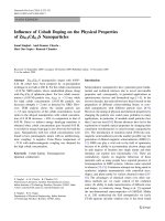
Apart from the quality of masonry units and mortar, the construction quality
also has a great effect on the quality of masonry structures. The limit strength
capacity and deformability of the masonry wall is affected by the quality of the
bonds between the masonry unit and mortar, i.e. the level of transfer of normal and
shear stresses in the contact surface (Fig. 1).
Compressive strength of masonry units or mortar is crucial for transfer of
normal compressive stresses r
n
on the contact surface. There is usually a differ-
ence in the strength capacity between the horizontal and vertical joints. Vertical
compressive stresses in masonry r
n,y
are usually much higher than horizontal
compressive stresses r
n,x
due to gravity load. In addition, the compressive strength
of horizontal joints is usually much higher than the compressive strength of ver-
tical joints. They are usually only partially filled with mortar, which, due to the
mode of placing, is usually of less strength than the mortar in horizontal joints.
The transfer of normal tensile stresses perpendicular to the joints is governed by
the adhesion between mortar and masonry unit.
The transfer of shear stresses in horizontal (s
x
) and vertical (s

y
) joints are also
different. The level of shear transfer in horizontal joints is greater than in vertical
joints because of higher quality and better adhesion between the mortar and the
masonry unit, especially due to the favourable effect of vertical compressive stress.
masonry unit
mortar
vertical joint
horizontal
joint
x
y
n,x
n,y
y
x
τ
τ
σ
σ
Fig. 1 Transfer of normal
(r
n
) and shear (s) stresses at
the joint of masonry units and
mortar
2 J. Radnic
´
et al.
The vertical holes through the masonry units contribute to masonry anisotropy.

The usual types of masonry walls are (Fig. 2):
1. Unreinforced masonry walls (Fig. 2a).
2. Reinforced masonry walls (Fig. 2b), with horizontal reinforcement in hori-
zontal joints and vertical reinforcement in the vertical holes through the
masonry units.
3. Confined masonry walls (Fig. 2c) are unreinforced masonry walls confined by
vertical and horizontal ring beams and foundation.
4. Subsequently constructed walls between the previously placed reinforced
concrete beams and columns (Fig. 2d)—the infilled frames.
A special confined masonry wall can often be found in practice. Here, classic
reinforced concrete columns and/or beams are constructed on part of the masonry
walls instead of vertical and/or horizontal ring beams (Fig. 2e).
(a)
(d) (e)
(b) (c)
vertical ring beam
foundation
horizontal ring beam
column
beam
phase II
phase I
foundation
reinforcement
reinforcement
horizontal ring beam
vertical ring beam
foundation
horizontal ring beam
beam

column
column
Fig. 2 Common types of masonry walls. a Unreinforced masonry. b Reinforced masonry.
c Confined masonry. d Masonry infilled framev. e Complex masonry
Numerical Model for Static and Dynamic Analysis of Masonry Structures 3
Masonry structures typically have a more complex behaviour and require more
complex engineering calculations and numerical models than pure concrete
structures.
Although there are many numerical models for static and dynamic analyses of
masonry structures (see for example [1–5]), there still is not a generally accepted
numerical model that would be sufficiently reliable and convenient for practical
applications. For a more realistic analysis of masonry structures, it is necessary to
include many nonlinear effects of the behaviour of the masonry, reinforced con-
crete and soil, such as:
• Yield of masonry in compression, opening of cracks in the masonry in tension,
mechanism of opening and closing of cracks under cyclic load, transfer of shear
stresses, anisotropic properties of strength and stiffness of masonry in horizontal
and vertical direction, tensile and shear stiffness of cracked masonry,
• Concrete yielding in compression, opening of cracks in concrete in tension,
mechanism of opening and closing of cracks in concrete under dynamic load,
tensile and shear stiffness of cracked concrete,
• Strain rate effect of the material properties of masonry, reinforced concrete and
soil,
• Soil yield under a foundation,
• Soil—structure dynamic interaction,
• Construction mode—the stages of masonry walls and infilled frames
assembling.
This chapter presents a numerical model for static and dynamic analyses of
planar (2D) masonry structures which include all previously mentioned nonlinear
effects in their behaviour.

2 Equilibrium Equation and Structure Discretization
2.1 Spatial Discretization
By the spatial discretization and application of the finite element method, the
equation of dynamic equilibrium of the masonry structure can be written as
follows:
M
€
u þ C
_
uðÞþRuðÞ¼f ð1Þ
where u are the unknown nodal displacements,
_
u are velocities and
€
u are accel-
eration; M is the mass matrix, C is the damping matrix and R(u) is a vector of
internal nodal forces; f is a vector of external nodal forces that can be generated by
wind, engines etc. ðf ¼ FðtÞÞ or by earthquakes ðf ¼ M
€
d
0
ðtÞÞÞ; see Fig. 3. Here,
€
d
0
is the base acceleration vector, and t is time. The inner forces vector R(u) can
be expressed as:
4 J. Radnic
´
et al.

RðuÞ¼Ku; K ¼ oR=ou ð2Þ
where K is the stiffness matrix of the structure.
To solve the eigen-problem, which is necessary in the dynamic analysis
(determination of the length of time increment for time integration of the equations
of motion), Eq. (1) is reduced to:
Kx ¼kx ð3Þ
where x is the eigen vector and k is the eigen value. The eigen-problem is solved
by the WYD method [6] (developed by Wilson, Yuan, and Dickens in 1982).
For static problems, Eq. (1) is reduced to
RuðÞ¼Ku ¼ f ð4Þ
where f is the vector of external static forces.
For spatial discretization of the structure, which is approximated by the state of
plane stress, 8-node (‘‘serendipity’’) elements are used (Fig. 4a). The structure
includes unreinforced or reinforced concrete, unreinforced or reinforced masonry,
and the soil under the foundation. Reinforcement within the 2D element is sim-
ulated using a 1D bar element. It is assumed that there is no slip between the
reinforcing bars and the surrounding concrete.
For contact modelling between the soil and foundations or between mortar and
masonry units, contact elements are used (Fig. 4b). Flat 2D six-node contact finite
elements of infinitely small thickness w (Fig. 4b1) can be used to simulate a
continuous connection between the basic 8-node elements, or 1D (bar) two-node
(a)
t

d
0
(b)
t
W
W

W

d
0
Fig. 3 Dynamic action on the masonry wall. a External force (wind, etc.). b Base acceleration
(earthquake)
Numerical Model for Static and Dynamic Analysis of Masonry Structures 5
contact elements (Fig. 4b2) for the simulation of the reinforcement which passes
across the contact surface.
2D contact elements can simulate sliding, separation and penetration of the
contact surface, based on the adopted material model of contact elements. 1D
contact elements can take the axial and shear forces, according to the adopted
material model.
2.2 Time Discretization
For the solution of Eq. (1), implicit, explicit or implicit-explicit Newmark algo-
rithms, developed in iterative form by Hughes [7], are used [8].
In the implicit algorithm, the equilibrium equation (1) is satisfied at the time
t
n+1
= t
n
? Dt, i.e. in (n ? 1) time step.
x
,
u
ζ,η
P( )
y
'
,

v
'
y
,
v
η
x
'
,
u
'
ζ
η=η
c
basic
element
reinforcement
(a)
b1 b2
w
basic element
2D contac element
basic element
i
j
w
1D contact element
basic element
basic elemen
t

(b)
Fig. 4 Adopted finite elements for the masonry structure. a Basic 2D eight-node (‘‘serendipity’’)
element for reinforced concrete, masonry and soil. b Contact elements between soil and
foundation or between mortar and masonry unit, b1 2D contact six-node element, b2 1D contact
two-node element
6 J. Radnic
´
et al.
M
€
u
nþ1
þ Ru
nþ1
;
_
u
nþ1
ðÞ¼f
nþ1
ð5Þ
where:
u
nþ1
¼ u
nþ1
þ bDt
2
€
u

n
_
u
nþ1
¼
_
u
nþ1
þ c Dt
€
u
n
ð6Þ
u
nþ1
¼ u
n
þ Dt
_
u
n
þ 0:5ð1 À 2bÞDt
2
€
u
n
_
u
nþ1
¼

_
u
n
þð1 À cÞ Dt
€
u
n
ð7Þ
In the above expressions, Dt is the time increment and n is the time step; u
nþ1
and
_
u
nþ1
are assumed, u
nþ1
and
_
u
nþ1
are corrected values of displacement and
velocity; b and c are parameters that determine the stability and accuracy of the
method [8].
By substituting (6) and (7) into (5), and by introducing an incremental-iterative
procedure to solve the general nonlinear problem, the so-called effective static
problem is obtained
K
Ã
s
Du ¼ðf

Ã
Þ
i
ð8Þ
where the effective tangent stiffness matrix K
Ã
s
is calculated at time s by:
K
Ã
s
¼
M
bDt
2
þ c
C
s
bDt
þ K
s
ð9Þ
and the effective load vector f
*
by:
f
Ã
¼ f
nþ1
À M

€
u
i
nþ1
À Rðu
i
nþ1
;
_
u
i
nþ1
Þð10Þ
In the above expressions, n indicates the time step, and i is the iterative step;
Du is the displacement increment vector. The Newmark implicit algorithm of the
iterative problem solution is shown in Table 1 [8].
The Newmark explicit algorithm of the iterative problem solution can be
written as follows:
M
€
u
nþ1
þ Ru
nþ1
+
_
u
nþ1
ðÞ¼f
nþ1

ð11Þ
This algorithm is shown in Table 2 [8]. In the explicit methods, the dynamic
equilibrium equation is satisfied in the time t
n
, and the unknown variables are
calculated in the time t
n+1
= t
n
? Dt.
The main advantage of this method is the small number and simple numerical
operations within each time step. Their main disadvantage is that they are not
unconditionally stable. Therefore, the calculating advantage of explicit methods is
often compensated by the fact that small time increments are required when solid
(small) elements are present in the system. These methods are often not effective in
the use of solid contact elements.
It is possible to use the implicit and explicit Newmark algorithms at the same
time [8]. Specifically, the area of the structure with rigid elements is effectively
Numerical Model for Static and Dynamic Analysis of Masonry Structures 7
integrated with the implicit algorithms, and the area of the structure with soft
elements with the explicit algorithm.
3 Material Model
The application of an adequate material model for a realistic simulation of the
behaviour of masonry structures under static and dynamic loads is of primary
importance. The material models applied here for certain parts of masonry
structures (reinforced concrete, masonry, soil) are described briefly hereinafter.
Table 1 Newmark implicit algorithm of the iterative problem solution
(1) For time step (n+1), use iterative step i = 1
(2) Calculate the vectors of the assumed displacement, velocity and acceleration at the beginning
of time step using the known values from previous time step:

u
1
nþ1
¼ u
nþ1
_
u
1
nþ1
¼
_
u
nþ1
€
u
1
nþ1
¼ u
1
nþ1
À u
nþ1
ÀÁ
bDt
2
ÀÁ
(3)
Calculate effective residual forces f
Ã
ðÞ

i
:
f
Ã
ðÞ
i
¼ f
nþ1
À M
€
u
i
nþ1
À Ru
i
nþ1
;
_
u
i
nþ1
ÀÁ
(4) Calculate the effective stiffness matrix K
Ã
s
(if required):
K
Ã
s
¼

M
bDt
2
þ c
C
s
bDt
þ K
s
(5)
Calculate the displacement increment vector Du
i
:
K
Ã
s
Du
i
¼ f
Ã
ðÞ
i
(6) Correct the assumed values of displacement, velocity and acceleration:
u
iþ1
nþ1
¼ u
i
nþ1
þ Du

i
nþ1
€
u
iþ1
nþ1
¼ u
iþ1
nþ1
À u
nþ1
ÀÁ
bDt
2
ÀÁ
_
u
iþ1
nþ1
¼
_
u
i
nþ1
þ c DtðÞ
€
u
iþ1
nþ1
(7) Control the convergence procedure:

• if Du
i
satisfies the convergence criterion
Du
i





u
iþ1
nþ1




e
n
proceed to the next time step (replace ‘‘n’’ with ‘‘n+1’’ and proceed to solution step (1)). The
solution in time t
nþ1
is:
u
nþ1
¼ u
iþ1
nþ1
_
u

nþ1
¼
_
u
iþ1
nþ1
€
u
nþ1
¼
€
u
iþ1
nþ1
• if the convergence criterion is not satisfied, the iteration procedure with correction of shear,
velocity and acceleration continues (replace ‘‘i’’ with ‘‘i+1’’, and proceed to solution step
(3)).
8 J. Radnic
´
et al.
3.1 Reinforced Concrete Model
The presented model is used to simulate the behaviour of parts of masonry
structures made of concrete or reinforced concrete (ring beams, foundations,
columns, beams, etc.). This model was previously developed for static and
dynamic analyses of conventional reinforced concrete structures [8] and will be
only briefly described.
3.1.1 Concrete Model
A simple concrete model, based on the basic parameters of concrete, has been
adopted to simulate problems where nonlinearities are primarily caused by con-
crete cracking in tension and by concrete yielding in compression. A graphic

presentation of the adopted concrete model is shown in Fig. 5.
A. Concrete model in compression
For the description of concrete behaviour in compression, the theory of plas-
ticity is used with a defined yield criterion, flow rule and crushing criterion [8]. It
Table 2 Newmark explicit algorithm of the iterative problem solution
(1) For time step (n+1), use iteration step i = 1
(2) Calculate the vectors of the assumed displacement, velocity and acceleration at the beginning
of time step using the known values from previous time step:
u
1
nþ1
¼ u
nþ1
_
u
1
nþ1
¼
_
u
nþ1
€
u
1
nþ1
¼ u
1
nþ1
À u
nþ1

ÀÁ
bDt
2
ðÞ
(3)
Calculate effective residual forces f
Ã
ðÞ
i
:
f
Ã
ðÞ
i
¼f
nþ1
À Ru
i
nþ1
;
_
u
i
nþ1
ÀÁ
(4) Calculate the effective stiffness matrix K
Ã
(if required):
K
Ã

¼
M
bDt
2
Note: Since the matrix mass M is constant, it is sufficient to calculate the effective stiffness
matrix K
Ã
only once at the start of the solution. It is also obvious that it should be b [0
(5)
Calculate the displacement increment vector Du
i
:
K
Ã
Du
i
¼ f
Ã
ðÞ
i
(6) Correct the assumed values of displacement, velocity and acceleration:
u
iþ1
nþ1
¼ u
i
nþ1
þ Du
i
nþ1

€
u
iþ1
nþ1
¼ u
iþ1
nþ1
À u
nþ1
ÀÁ
bDt
2
ÀÁ
_
u
iþ1
nþ1
¼
_
u
i
nþ1
þ cDtðÞ
€
u
iþ1
nþ1
(7) Control the convergence procedure
In the explicit procedure with a single correction of the results, convergence control is not
required, but we directly proceed to the next time step

With multiple correction results it is necessary to control the procedure convergence, as
described in Table 1
Numerical Model for Static and Dynamic Analysis of Masonry Structures 9
is assumed that concrete under low stress levels is homogeneous and isotropic and
that the stress–strain relationship is linear-elastic. The relation between stress
increment Dr
c
and strain increment De
c
is expressed as:
Dr
c
¼ D
c
De
c
ð12Þ
where D
c
is the matrix of elastic concrete parameters. Linear-elastic behaviour is
valid until the yield condition is reached. Due to the simplicity, the Von Mises
yield criterion is used which is expressed through the stress components
Fðr
c
Þ¼ðr
2
x
þ r
2
y

À r
x
r
y
þ 3s
2
xy
Þ
1=2
À f
c;c
¼ 0 ð13Þ
where f
c,c
is the equivalent uniaxial concrete compressive strength. After the yield
criterion has been reached (13), an ideally plastic behaviour is adopted.
The concrete crushing criterion is defined as a function of strain components, as
F
e
ðe
c
Þ¼ðe
2
x
þ e
2
y
À e
x
e

y
þ 0:75c
2
xy
Þ
1=2
À e
c;c
¼ 0 ð14Þ
where e
c,c
is the equivalent uniaxial ultimate compressive strain of concrete
(values between 0.0035 and -0.005 are usually used). When the crushing con-
dition is reached, it is assumed that the concrete has no stiffness. The concrete
failure in one or more integration points does not mean the failure of the whole
structure.
B. Tension concrete model
Initially, the linear-elastic behaviour is assumed until the criterion of cracks
initiation is reached
r
1
!f
c;t
and/or r
2
!f
c;t
ð15Þ
2
σ

yielding
axis of symmetry
compression-compression
yielding
σ
1
=
tension-compression
cracking
cracking
compression-tension
f
c,c
c,t
f
tension-tension
σ
1
2
σ
c,t
f
c,c
f
ε
c
σ
c
tension
compression

c,t
f
c,t
f
α
c
E
c,c
f
ε
c
,
t
ε
c
,
c
cracking
yielding
crushing
(a)
(b)
cracking
cracking
Fig. 5 Graphic presentation of the adopted concrete model. a 1D model. b 2D model
10 J. Radnic
´
et al.
in the tension–tension area
ðf

c;t
À r
1
Þ=f
c;t
!r
2
=f
c;c
or r
1
f
c;c
þ r
2
f
c;t
f
c;c
f
c;t
ð16Þ
in the tension–compression area. It is assumed that the cracks occur in the plane
perpendicular to the direction of principal stresses r1, r2, and that after their
occurrence the concrete remains continuum.
The cracks are modelled as smeared, which disregards the actual displacement
discontinuity and the topology of the idealized structure remains unchanged after
concrete cracking. After opening of cracks, it is assumed that the cracks position
remains unchanged for the next loading and unloading. After opening of cracks,
the concrete becomes anisotropic and the crack direction determines the main

directions of concrete anisotropy. Partial or full closing of previously open cracks
is modelled, as well as reopening of previously closed cracks. The transfer of
compressive stress across a fully closed crack is modelled as for concrete without
cracks. After crack reopening, the tensile stiffness of cracked concrete is not
considered any more. Possible states of concrete cracks are shown in Fig. 6. The
crack model is shown in Fig. 7.
The stress–strain relationship of cracked concrete can be expressed as:
r
Ã
c
¼ D
Ã
c
e
Ã
c
ð17Þ
where D
Ã
c
is the matrix of ‘‘elastic’’ constants of the cracked concrete. The com-
ponents of the stress vector r
Ã
c
¼ r
Ã
n
; r
Ã
t

; s
Ã
nt
ÂÃ
T
and strain vector e
Ã
c
¼ e
Ã
n
; e
Ã
t
; e
Ã
nt
ÂÃ
T
are in accordance with the local coordinate system (Fig. 7c).
For the plane stress state, the stress–strain relationship for concrete with one
crack in the direction of the y* axis is
r
Ã
n
r
Ã
t
s
Ã

nt
2
4
3
5
¼
00 0
0 E
c
0
00G
Ã
c
2
4
3
5
e
Ã
n
e
Ã
t
c
Ã
nt
2
4
3
5

ð18Þ
Without of cracks First crack opened First crack closed
First crack still closed
Second crack o
p
ened
Both cracks closed Both cracks opened
Fig. 6 Crack pattern in
concrete
Numerical Model for Static and Dynamic Analysis of Masonry Structures 11
For concrete with two cracks, the matrix D
Ã
c
is
D
Ã
c
¼
00 0
00 0
00G
Ã
c
2
4
3
5
ð19Þ
where E
c

is the elasticity modulus of concrete and G
Ã
c
is the modified shear
modulus of cracked concrete.
B.1 Modelling of the tensile stiffness of the cracked concrete
The tensile stiffness of the cracked concrete is simulated by gradual decrease of
the tensile stress components perpendicular to the crack, in accordance with the
stress–strain relationship for the uniaxial stress state (Fig. 8). When the crack
opens, where r
1
¼ f
c;t
¼ E
c
e
cr
; the normal stress perpendicular to the crack
decreases to r
Ã
n
¼ af
c;t
: When the strain perpendicular to the crack exceeds e
c;t
;
r
Ã
n
¼ 0 is adopted. The ultimate strain e

c;t
is
e
c;t
¼ ae
cr
ð20Þ
where e
cr
is the strain at crack opening, and a is an adopted parameter (usually 5–25).
B.2 Modelling of the shear stiffness of the cracked concrete
In accordance with the adopted smeared crack model, the shear modulus of
concrete G
c
is linearly reduced depending on the value of tensile concrete strain
perpendicular to the crack e
Ã
n
: Specifically, the shear modulus of cracking concrete
G
Ã
c
is defined by (Fig. 9)
G
Ã
c
¼
"
bG
c

ð21Þ
where
b is a parameter defined by
σ
y
τ
x
y
x
y
τ
σ
x
x
y
τ
x
σ
x
y
τ
y
σ
α
c
r
c
r
α
y

x
y
x
2
σ
2
σ
σ
1
σ
1
c
r
α
∗
∗
∗
(a) (b)
E
c
=0
=0
E
c
/
(c)
σ
τ
x
y

x
y
x
τ
σ
y
c
r
α
x
y
τ
x
σ
x
y
τ
σ
y
σ
t
∗
∗
t
σ
σ
n
∗
σ
n

∗
∗
∗
∗
∗
∗
∗
∗
∗
∗
τ
τ
∗
∗
τ
τ
∗
σ
1
= f
c
,
t
σ
1
2
σ
1
σ
σ

2
Fig. 7 Concrete cracks model. a Principal stress direction. b Crack direction. c Stresses after
cracking
12 J. Radnic
´
et al.
b ¼ 1 Àe
Ã
n
=e
c;p
for e
Ã
n
e
c;p
b ¼ 0 for e
Ã
n
[ e
c;p
ð22Þ
where e
c;p
is the ultimate strain perpendicular to the concrete crack over which
there is no aggregate interlocking, i.e. over which there is no shear transfer. It can
be written as
e
c;p
¼ ce

cr
ð23Þ
The empirical parameter
c is usually between 10 and 35, i.e. e
c;p
is usually
between 0.001 and 0.004 [8].
(b)
(c)
c
r
ε
σ
c
,
t
f
c
c
,
t
ε
c
ε
ε
=
c
,
t
α

c
,
t
ε
ε
c
r
c
,
t
c
,
t
α
f
f
ε
n+1
c
r
ε
ε
n
n+1
σ
σ
c
c
n
c

,
t
ε
σ
ε
c
(a)
α
f
c
,
t
ε
c
r
c
E
f
c
,
t
c
E =0
c
σ
ε
Fig. 8 Stress-strain relationship for concrete after crack opening. a Crack opening. b Crack
closure. c Crack re-opening
c
,

p
ε
n
ε
1.0
c
,
p
ε
=
β
ε
c
r
0.0
γ
*
ε
*
β
=G /G
cc
*
Fig. 9 Shear stiffness model
of the cracked concrete
Numerical Model for Static and Dynamic Analysis of Masonry Structures 13
3.1.2 Reinforcement Model
The reinforcement is simulated by a bar element within the concrete element
(Fig. 4a). The adopted stress–strain relationship for the reinforcement is shown in
Fig. 10. Here f

s;c
and f
s;t
are the uniaxial compressive and tensile steel strengths;
e
s;c
and e
s;t
are the uniaxial compressive and tensile limit steel strains; E
s
and E
0
s
are
the elasticity steel modules.
3.2 Masonry Model
3.2.1 Introduction
In the static and dynamic analyses of masonry structures, two numerical models
for masonry are commonly used: macro model and micro model (Fig. 11).
(i) Macro model of masonry (Fig. 11b). At the macro level, the masonry is
approximated by a representative material whose physical–mechanical prop-
erties describe the actual complex masonry properties. Such an approach
allows large finite elements (rough discretization) and significantly reduces the
number of unknown variables, and also rapidly accelerates the structure
analysis.
(ii) Micro model of masonry (Fig. 11c). At the micro level, the spatial discreti-
zation of masonry can be performed at the level of masonry units and mortar
(joints). For a more accurate analysis, the connection between mortar and
masonry units can be simulated by contact elements. It is possible to use
various micro models of masonry, with various precision and duration of

analysis. In relation to the masonry macro model, the masonry micro models
can provide a more accurate description of the damage and failure of masonry,
but with much more complex analysis. It is used mainly for smaller spatial
problems, and for verification of experimental tests of the masonry structures.
σ
E
s
ε
s
s
s
E'
s,t
ε
ε
s,c
s
E
failure
s
E'
failure
s,c
f
E
s
f
s,t
s
E

s,t
f
s,c
f
Fig. 10 Stress-strain
relationship for the
reinforcement
14 J. Radnic
´
et al.
The adopted macro model and micro models of masonry are briefly described
hereinafter.
3.2.2 Macro Model of Masonry
In this model, attention should be given to defining the adequate physical–
mechanical parameters of a representative idealized material. This material should
describe the complex structures of masonry units, mortar in the joints and the
connection characteristics between the mortar and masonry units.
The adopted constitutive model can simulate anisotropic properties of masonry,
with different elasticity modulus E
m
; strength (compressive f
m;c
; tensile f
m;t
; shear
f
m;p
) and limit strains (compressive e
m;c
; tensile e

m;t
) for horizontal (h) and vertical
(v) directions (Fig. 12). The correspondent parameters for the representative
material are determined based on analysis of relevant data for masonry units,
mortar and connections between mortar and masonry units.
A. Modelling of masonry in compression and tension
A graphic presentation of the adopted orthotropic constitutive masonry model in
compression and tension is given in Fig. 13. The masonry parameters in the hori-
zontal (h) and vertical (v) directions are: r
h
m
and r
v
m
are normal stresses, f
h
m;c
and
horizontal
joint
vertcal joint
masonry units
mortar
finite elements of the equivalent material
finite elements for the masonry units
finite elements for the mortar
contact elements between the masonry units and morta
r
finite element for the masonry units
(b)

(a)
(c1)
(c2)
(c)
finite element for the mortar
Fig. 11 Macro and micro models of masonry. a Fragmentof masonry. b Macro model of masonry.
c Micro models of masonry, c1 Micro model of masonry 1, c2 Micro model of masonry 2
Numerical Model for Static and Dynamic Analysis of Masonry Structures 15
f
v
m;c
are the compressive strengths, f
h
m;t
and f
v
m;t
are the tensile strengths, E
h
m
and E
v
m
are the elasticity modules, e
h
m;c
and e
v
m;c
are the crushing compressive strains.

As shown in Fig. 13, the effect of biaxial stresses to the limit compressive
strength of masonry walls is disregarded. This effect could be easily included if the
experimental results of the strength of walls with different proportions of normal
stresses were known. In real masonry structures, the basic parameters of the masonry
in the vertical direction have higher values than in the horizontal direction.
If there are no experimental values for the compressive masonry strength, then
the smaller value of the respective compressive strengths of the masonry unit or
mortar in vertical and horizontal directions can be used. Also, if there are no
v (vertical)
h (horizontal)
masonry unit
horizontal joint
vertcal joint
equivalent material
E , f , f ,
mo
mo,c
mo,t
mo,c
v
v
h
eight - node
finite element
(b)
(a)
v
h
ε
v

v
v
E , f , f ,
mo
mo,c
mo,t
mo,c
h
ε
h
h
h
E , f , f ,
e e,c e,t e,c
vv v
v
E , f , f ,
ee,ce,t
e,c
hh
h
h
ε
ε
E , f , f ,
mm,c
m,t
m,c
vv v
v

ε
E , f , f ,
m m,c m,t m,c
hh h
h
ε
Fig. 12 Parameters of
orthotropic masonry.
a Fragment of real masonry
with parameters for masonry
units and mortar. b Macro
model of masonry with the
parameters of the equivalent
material
yielding
compression-compression
yielding
tension-compression
compression-tension
f
m,c
m,t
f
tension-tension
σ
m
m
σ
m,t
f

m,c
f
(a) (b)
cracking
cracking
v
h
v
h
v
h
v (vertical)
h (horizontal)
m,t
f
m,t
f
m
E
m,c
f
ε
m
ε
m,c
cracking
yielding
crushing
v
crushing

m
E
h
v
h
m
f
v
m,c
f
h
v
ε
m,c
h
cracking
vertical direction
horizontal direction
ε
m.t
v
ε
m,t
h
Fig. 13 Adopted orthotropic masonry model. a 2D model. b 1D model
16 J. Radnic
´
et al.
experimental values for the tensile masonry strength, then the adhesion strength
between mortar and masonry units in vertical and horizontal joints can be used.

The masonry model in tension after cracking is used as in concrete (Fig. 8). It is
possible to simulate the tensile stiffness of cracked masonry. The value of
parameter
a for the masonry, which determines the maximum tensile strain per-
pendicular to the crack over which there is no tensile stiffness of the masonry,
should be determined experimentally.
Cracks modelling of masonry are analogous to that for concrete, where,
according to the adopted assumption, the cracks in the masonry are horizontal and/
or vertical (Fig. 14). The transmission of compression stresses over the closed
crack is modelled as in homogeneous masonry. After re-opening of the previously
closed crack, the stiffness of the masonry is not taken into account. After crushing
in compression, it is assumed that the masonry has no stiffness.
B. Modelling of masonry shear failure
Apart from tension (cracking) and/or compression (crushing), the collapse of
the masonry due to the shear stress in the horizontal plane (horizontal joint) is
modelled. Shear failure in the vertical joint is not currently modelled. The criterion
of the masonry shear failure in the horizontal plane is defined according to Fig. 15,
or as
s
xy
s
h
m
ð24Þ
where s
xy
is the masonry shear stress from the numerical calculation, and s
h
m
is the

masonry shear strength defined with (compressive stress has a negative sign)
Without of cracks First crack opened First crack closed
First crack still closed
Second crack o
p
ened
Both cracks closed
Both cracks opened
Fig. 14 Cracks pattern of
masonry
Numerical Model for Static and Dynamic Analysis of Masonry Structures 17
(i) r
v
0 (compression)
s
h
m
¼ s
h
m;0
À 0:4r
v
m
s
h
m;g
¼ s
h
m;0
À 0:4f

t
m;c
ð25Þ
(ii) r
v
[ 0 (tension)
s
h
m
¼ s
h
m;0
1 À
r
v
m
f
v
m;t
!
!0 ð26Þ
In the previous expressions, s
h
m;0
is the basic masonry shear strength (without
normal compressive stresses transversal to the horizontal joints), and r
v
m
is the
vertical stress.

The shear stiffness of cracked masonry is simulated similarly to the shear
stiffness of cracked concrete. Specifically, assuming that after cracking masonry
remains a continuum, the initial shear modulus G
m
of the masonry is reduced
according to the value of the tensile strain perpendicular to the crack e
Ã
n;m
;
according to (Fig. 16)
G
Ã
m
¼ bG
m
ð27Þ
where G
Ã
m
is the shear modulus of cracked masonry and b is a parameter defined by
"
"
b ¼ 1 À
e
Ã
n;m
e
m;p
for e
Ã

n;m
e
m;p
"
"
b ¼ 0 for e
Ã
n;m
[ e
m;p
ð28Þ
where e
m;p
is the limit strain perpendicular to the crack where there is no transfer of
shear stress. It can be written as follows:
e
m;p
¼ c=e
mr
ð29Þ
m,0
τ
h
m,c
f
0.4
m,g
τ
h
m,0

τ
h
cracking
m,t
f
v
1
0.4
m
σ
v
(tension)
(compression)
shear failure
m
τ
h
crushing
m,c
f
Fig. 15 Adopted shear
failure of masonry
18 J. Radnic
´
et al.
Parameter c should be experimentally determined for various types of masonry
and load types. In case of shear failure of the masonry in a certain integration
point, i.e. when s
x;y
[ s

h
m;g
,G
m
= 0 is adopted.
3.2.3 Micro Model of Masonry
The masonry can be more precisely and reliably modelled by the micro model than
by the macro model. It is possible to use various micro models of masonry (some
of them are presented in Fig. 11), with various precision and duration of analysis.
In micro model 1 in Fig. 11, the masonry units and mortar are discretized by 8-
node elements, while at the contact of mortar and masonry units, thin 6-node
contact elements are used. The constitutive material models of all these elements
can well describe all effects of materials and contact surfaces.
In micro model 2 in Fig. 11, masonry units are discretized by 8-node elements,
and vertical and horizontal joints with 6-node contact elements.
Also, other micro models can be used, i.e. different discretization of masonry.
3.3 Contact Element Model
2D contact elements transmit normal stress r
n
at the contact surface according to
Fig. 17, which allows simulation of sliding, separation and penetration at the
contact surface between the foundation and soil, or between the mortar and the
masonry units. It is possible to define different types of r
n
À e
n
relationships,
where r
n
is the stress and e

n
is the strain perpendicular to the contact surface.
In compression, r
k;c
denotes the compressive strength at the contact surface, e
k;c
is the ultimate compressive strain at failure, E
k
is the elasticity modulus perpen-
dicular to the contact surface and E
1
is the hardening modulus.
In tension, r
k;t
denotes the tensile strength over which cracks occur, E
2
is the
hardening modulus, e
k;t
is the tensile strain perpendicular to the contact surface
when cracks occur, and e
k;g
is the maximum tensile strain perpendicular to the
contact surface over which there is no tensile stiffness. The model of tensile
m,p
ε
1.0
0.0
ε
*

β
=G /G
mm
*
n,m
Fig. 16 Adopted shear
stiffness of cracked masonry
Numerical Model for Static and Dynamic Analysis of Masonry Structures 19