Báo cáo khoa học: "How to train your multi bottom-up tree transducer" potx

Proceedings of the 49th Annual Meeting of the Association for Computational Linguistics, pages 825–834,
Portland, Oregon, June 19-24, 2011.
c
2011 Association for Computational Linguistics
How to train your multi bottom-up tree transducer
Andreas Maletti
Universit
¨
at Stuttgart, Institute for Natural Language Processing
Azenbergstraße 12, 70174 Stuttgart, Germany

Abstract
The local multi bottom-up tree transducer is
introduced and related to the (non-contiguous)
synchronous tree sequence substitution gram-
mar. It is then shown how to obtain a weighted
local multi bottom-up tree transducer from
a bilingual and biparsed corpus. Finally,
the problem of non-preservation of regular-
ity is addressed. Three properties that ensure
preservation are introduced, and it is discussed
how to adjust the rule extraction process such
that they are automatically fulfilled.
1 Introduction
A (formal) translation model is at the core of ev-
ery machine translation system. Predominantly, sta-
tistical processes are used to instantiate the for-
mal model and derive a specific translation device.
Brown et al. (1990) discuss automatically trainable
translation models in their seminal paper. However,
the IBM models of Brown et al. (1993) are string-

based in the sense that they base the translation de-
cision on the words and their surrounding context.
Contrary, in the field of syntax-based machine trans-
lation, the translation models have full access to the
syntax of the sentences and can base their decision
on it. A good exposition to both fields is presented
in (Knight, 2007).
In this paper, we deal exclusively with syntax-
based translation models such as synchronous tree
substitution grammars (STSG), multi bottom-up tree
transducers (MBOT), and synchronous tree-sequence
substitution grammars (STSSG). Chiang (2006)
gives a good introduction to STSG, which originate
from the syntax-directed translation schemes of Aho
and Ullman (1972). Roughly speaking, an STSG
has rules in which two linked nonterminals are re-
placed (at the same time) by two corresponding trees
containing terminal and nonterminal symbols. In
addition, the nonterminals in the two replacement
trees are linked, which creates new linked nontermi-
nals to which further rules can be applied. Hence-
forth, we refer to these two trees as input and output
tree. MBOT have been introduced in (Arnold and
Dauchet, 1982; Lilin, 1981) and are slightly more
expressive than STSG. Roughly speaking, they al-
low one replacement input tree and several output
trees in a single rule. This change and the pres-
ence of states yields many algorithmically advanta-
geous properties such as closure under composition,
efficient binarization, and efficient input and output

restriction [see (Maletti, 2010)]. Finally, STSSG,
which have been derived from rational tree rela-
tions (Raoult, 1997), have been discussed by Zhang
et al. (2008a), Zhang et al. (2008b), and Sun et al.
(2009). They are even more expressive than the lo-
cal variant of the multi bottom-up tree transducer
(LMBOT) that we introduce here and can have sev-
eral input and output trees in a single rule.
In this contribution, we restrict MBOT to a form
that is particularly relevant in machine translation.
We drop the general state behavior of MBOT and re-
place it by the common locality tests that are also
present in STSG, STSSG, and STAG (Shieber and
Schabes, 1990; Shieber, 2007). The obtained device
is the local MBOT (LMBOT).
Maletti (2010) argued the algorithmical advan-
tages of MBOT over STSG and proposed MBOT as
an implementation alternative for STSG. In partic-
ular, the training procedure would train STSG; i.e.,
it would not utilize the additional expressive power
825
of MBOT. However, Zhang et al. (2008b) and Sun
et al. (2009) demonstrate that the additional expres-
sivity gained from non-contiguous rules greatly im-
proves the translation quality. In this contribution
we address this separation and investigate a training
procedure for LMBOT that allows non-contiguous
fragments while preserving the algorithmic advan-
tages of MBOT. To this end, we introduce a rule ex-
traction and weight training method for LMBOT that

is based on the corresponding procedures for STSG
and STSSG. However, general LMBOT can be too
expressive in the sense that they allow translations
that do not preserve regularity. Preservation of reg-
ularity is an important property for efficient repre-
sentations and efficient algorithms [see (May et al.,
2010)]. Consequently, we present 3 properties that
ensure that an LMBOT preserves regularity. In addi-
tion, we shortly discuss how these properties could
be enforced in the rule extraction procedure.
2 Notation
The set of nonnegative integers is N. We write [k]
for the set {i | 1 ≤ i ≤ k}. We treat functions as
special relations. For every relation R ⊆ A × B and
S ⊆ A, we write
R(S) = {b ∈ B | ∃a ∈ S : (a, b) ∈ R}
R
−1
= {(b, a) | (a, b) ∈ R} ,
where R
−1
is called the inverse of R.
Given an alphabet Σ, the set of all words (or se-
quences) over Σ is Σ
∗
, of which the empty word is ε.
The concatenation of two words u and w is simply
denoted by the juxtaposition uw. The length of a
word w = σ
1

· · · σ
k
with σ
i
∈ Σ for all i ∈ [k]
is |w| = k. Given 1 ≤ i ≤ j ≤ k, the (i, j)-
span w[i, j] of w is σ
i
σ
i+1
· · · σ
j
.
The set T
Σ
of all Σ-trees is the smallest set T
such that σ(t) ∈ T for all σ ∈ Σ and t ∈ T
∗
.
We generally use bold-face characters (like t) for
sequences, and we refer to their elements using sub-
scripts (like t
i
). Consequently, a tree t consists of
a labeled root node σ followed by a sequence t of
its children. To improve readability we sometimes
write a sequence t
1
· · · t
k

as t
1
, . . . , t
k
.
The positions pos(t) ⊆ N
∗
of a tree t = σ(t) are
inductively defined by pos(t) = {ε}∪pos(t), where
pos(t) =

1≤i≤|t|
{ip | p ∈ pos(t
i
)} .
Note that this yields an undesirable difference be-
tween pos(t) and pos(t), but it will always be clear
from the context whether we refer to a single tree or
a sequence. Note that positions are ordered via the
(standard) lexicographic ordering. Let t ∈ T
Σ
and
p ∈ pos(t). The label of t at position p is t(p), and
the subtree rooted at position p is t|
p
. Formally, they
are defined by
t(p) =

σ if p = ε

t(p) otherwise
t(ip) = t
i
(p)
t|
p
=

t if p = ε
t|
p
otherwise
t|
ip
= t
i
|
p
for all t = σ(t) and 1 ≤ i ≤ |t|. As demonstrated,
these notions are also used for sequences. A posi-
tion p ∈ pos(t) is a leaf (in t) if p1 /∈ pos(t). Given
a subset NT ⊆ Σ, we let
↓
NT
(t) = {p ∈ pos(t) | t(p) ∈ NT, p leaf in t} .
Later NT will be the set of nonterminals, so that
the elements of ↓
NT
(t) will be the leaf nonterminals
of t. We extend the notion to sequences t by

↓
NT
(t) =

1≤i≤|t|
{ip | p ∈ ↓
NT
(t
i
)} .
We also need a substitution that replaces sub-
trees. Let p
1
, . . . , p
n
∈ pos(t) be pairwise in-
comparable positions and t
1
, . . . , t
n
∈ T
Σ
. Then
t[p
i
← t
i
| 1 ≤ i ≤ n] denotes the tree that is ob-
tained from t by replacing (in parallel) the subtrees
at p

i
by t
i
for every i ∈ [k].
Finally, let us recall regular tree languages. A fi-
nite tree automaton M is a tuple (Q, Σ, δ, F ) such
that Q is a finite set, δ ⊆ Q
∗
× Σ × Q is a fi-
nite relation, and F ⊆ Q. We extend δ to a map-
ping δ : T
Σ
→ 2
Q
by
δ(σ(t)) = {q | (q, σ, q) ∈ δ, ∀i ∈ [ |t| ]: q
i
∈ δ(t
i
)}
for every σ ∈ Σ and t ∈ T
∗
Σ
. The finite tree automa-
ton M recognizes the tree language
L(M) = {t ∈ T
Σ
| δ(t) ∩ F = ∅} .
A tree language L ⊆ T
Σ

is regular if there exists a
finite tree automaton M such that L = L(M).
826
VP
VBD
signed
PP
→
PV
twlY
,
NP-OBJ
NP
DET-NN
AltwqyE
PP
1
S
NP-SBJ
VP
→
VP
PV
NP-OBJ NP-SBJ
1
2
1
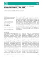
Figure 1: Sample LMBOT rules.
3 The model
In this section, we recall particular multi bottom-

up tree transducers, which have been introduced
by Arnold and Dauchet (1982) and Lilin (1981). A
detailed (and English) presentation of the general
model can be found in Engelfriet et al. (2009) and
Maletti (2010). Using the nomenclature of Engel-
friet et al. (2009), we recall a variant of linear and
nondeleting extended multi bottom-up tree transduc-
ers (MBOT) here. Occasionally, we will refer to gen-
eral MBOT, which differ from the local variant dis-
cussed here because they have explicit states.
Throughout the article, we assume sets Σ and ∆
of input and output symbols, respectively. More-
over, let NT ⊆ Σ ∪ ∆ be the set of designated non-
terminal symbols. Finally, we avoid weights in the
formal development to keep it simple. It is straight-
forward to add weights to our model.
Essentially, the model works on pairs t, u
consisting of an input tree t ∈ T
Σ
and a se-
quence u ∈ T
∗
∆
of output trees. Each such pair is
called a pre-translation and the rank rk(t, u) the
pre-translation t, u is |u|. In other words, the rank
of a pre-translation equals the number of output trees
stored in it. Given a pre-translation t, u ∈ T
Σ
×T

k
∆
and i ∈ [k], we call u
i
the i
th
translation of t. An
alignment for the pre-translation t, u is an injec-
tive mapping ψ: ↓
NT
(u) → ↓
NT
(t) × N such that
(p, j) ∈ ψ(↓
NT
(u)) for every (p, i) ∈ ψ(↓
NT
(u))
and j ∈ [i]. In other words, an alignment should re-
quest each translation of a particular subtree at most
once and if it requests the i
th
translation, then it
should also request all previous translations.
Definition 1 A local multi bottom-up tree trans-
ducer (LMBOT) is a finite set R of rules such that ev-
ery rule, written l →
ψ
r, contains a pre-translation
l, r and an alignment ψ for it.

The component l is the left-hand side, r is
the right-hand side, and ψ is the alignment of a
rule l →
ψ
r ∈ R. The rules of an LMBOT are similar
to the rules of an STSG (synchronous tree substitu-
tion grammar) of Eisner (2003) and Shieber (2004),
but right-hand sides of LMBOT contain a sequence
of trees instead of just a single tree as in an STSG. In
addition, the alignments in an STSG rule are bijec-
tive between leaf nonterminals, whereas our model
permits multiple alignments to a single leaf nonter-
minal in the left-hand side. A model that is even
more powerful than LMBOT is the non-contiguous
version of STSSG (synchronous tree-sequence sub-
stitution grammar) of Zhang et al. (2008a), Zhang
et al. (2008b), and Sun et al. (2009), which al-
lows sequences of trees on both sides of rules [see
also (Raoult, 1997)]. Figure 1 displays sample rules
of an LMBOT using a graphical representation of the
trees and the alignment.
Next, we define the semantics of an LMBOT R.
To avoid difficulties
1
, we explicitly exclude rules
like l →
ψ
r where l ∈ NT or r ∈ NT
∗
; i.e.,

rules where the left- or right-hand side are only
leaf nonterminals. We first define the traditional
bottom-up semantics. Let ρ = l →
ψ
r ∈ R be a
rule and p ∈ ↓
NT
(l). The p-rank rk(ρ, p) of ρ is
rk(ρ, p) = |{i ∈ N | (p, i) ∈ ψ(↓
NT
(r))}|.
Definition 2 The set τ (R) of pre-translations of an
LMBOT R is inductively defined to be the smallest
set such that: If ρ = l →
ψ
r ∈ R is a rule,
t
p
, u
p
 ∈ τ (R) is a pre-translation of R for every
p ∈ ↓
NT
(l), and
• rk(ρ, p) = rk(t
p
, u
p
),
• l(p) = t

p
(ε), and
1
Actually, difficulties arise only in the weighted setting.
827
PP
IN
for
NP
NNP
Serbia

PP
PREP
En
NP
NN-PROP
SrbyA

VP
VBD
signed
PP
IN
for
NP
NNP
Serbia

PV

twlY
,
NP-OBJ
NP
DET-NN
AltwqyE
PP
PREP
En
NP
NN-PROP
SrbyA

S
. . .
VP
VBD
signed
PP
IN
for
NP
NNP
Serbia

VP
PV
twlY
NP-OBJ
NP

DET-NN
AltwqyE
PP
PREP
En
NP
NN-PROP
SrbyA
. . .

Figure 2: Top left: (a) Initial pre-translation; Top right: (b) Pre-translation obtained from the left rule of Fig. 1 and (a);
Bottom: (c) Pre-translation obtained from the right rule of Fig. 1 and (b).
• r(p

) = u
p

(i) with ψ(p

) = (p

, i)
for every p

∈ ↓
NT
(r), then t, u ∈ τ(R) where
• t = l[p ← t
p
| p ∈ ↓

NT
(l)] and
• u = r[p

← (u
p

)
i
| p

∈ ψ
−1
(p

, i)].
In plain words, each nonterminal leaf p in the
left-hand side of a rule ρ can be replaced by the
input tree t of a pre-translation t, u whose root
is labeled by the same nonterminal. In addition,
the rank rk(ρ, p) of the replaced nonterminal should
match the rank rk(t, u) of the pre-translation and
the nonterminals in the right-hand side that are
aligned to p should be replaced by the translation
that the alignment requests, provided that the non-
terminal matches with the root symbol of the re-
quested translation. The main benefit of the bottom-
up semantics is that it works exclusively on pre-
translations. The process is illustrated in Figure 2.
Using the classical bottom-up semantics, we sim-

ply obtain the following theorem by Maletti (2010)
because the MBOT constructed there is in fact an
LMBOT.
Theorem 3 For every STSG, an equivalent LMBOT
can be constructed in linear time, which in turn
yields a particular MBOT in linear time.
Finally, we want to relate LMBOT to the STSSG
of Sun et al. (2009). To this end, we also introduce
the top-down semantics for LMBOT. As expected,
both semantics coincide. The top-down semantics is
introduced using rule compositions, which will play
an important rule later on.
Definition 4 The set R
k
of k-fold composed rules is
inductively defined as follows:
• R
1
= R and
•  →
ϕ
s ∈ R
k+1
for all ρ = l →
ψ
r ∈ R and
ρ
p
= l
p

→
ψ
p
r
p
∈ R
k
such that
– rk(ρ, p) = rk(l
p
, r
p
),
– l(p) = l
p
(ε), and
– r(p

) = r
p

(i) with ψ(p

) = (p

, i)
for every p ∈ ↓
NT
(l) and p


∈ ↓
NT
(r) where
–  = l[p ← l
p
| p ∈ ↓
NT
(l)],
– s = r[p

← (r
p

)
i
| p

∈ ψ
−1
(p

, i)], and
– ϕ(p

p) = p

ψ
p

(ip) for all positions

p

∈ ψ
−1
(p

, i) and ip ∈ ↓
NT
(r
p

).
The rule closure R
≤∞
of R is R
≤∞
=

i≥1
R
i
. The
top-down pre-translation of R is
τ
t
(R) = {l, r  | l →
ψ
r ∈ R
≤∞
, ↓

NT
(l) = ∅} .
828
X
X
→
X
a
X
,
X
a
X
1
2
X
X
→
X
b
X
,
X
b
X
1
2
X
X
X

→
X
a
X
b
X
,
X
a
X
b
X
1
2
Figure 3: Composed rule.
The composition of the rules, which is illus-
trated in Figure 3, in the second item of Defini-
tion 4 could also be represented as ρ(ρ
1
, . . . , ρ
k
)
where ρ
1
, . . . , ρ
k
is an enumeration of the rules
{ρ
p
| p ∈ ↓

NT
(l)} used in the item. The follow-
ing theorem is easy to prove.
Theorem 5 The bottom-up and top-down semantics
coincide; i.e., τ(R) = τ
t
(R).
Chiang (2005) and Graehl et al. (2008) argue that
STSG have sufficient expressive power for syntax-
based machine translation, but Zhang et al. (2008a)
show that the additional expressive power of tree-
sequences helps the translation process. This is
mostly due to the fact that smaller (and less specific)
rules can be extracted from bi-parsed word-aligned
training data. A detailed overview that focusses on
STSG is presented by Knight (2007).
Theorem 6 For every LMBOT, an equivalent STSSG
can be constructed in linear time.
4 Rule extraction and training
In this section, we will show how to automatically
obtain an LMBOT from a bi-parsed, word-aligned
parallel corpus. Essentially, the process has two
steps: rule extraction and training. In the rule ex-
traction step, an (unweighted) LMBOT is extracted
from the corpus. The rule weights are then set in the
training procedure.
The two main inspirations for our rule extraction
are the corresponding procedures for STSG (Galley
et al., 2004; Graehl et al., 2008) and for STSSG (Sun
et al., 2009). STSG are always contiguous in both

the left- and right-hand side, which means that they
(completely) cover a single span of input or output
words. On the contrary, STSSG rules can be non-
contiguous on both sides, but the extraction proce-
dure of Sun et al. (2009) only extracts rules that are
contiguous on the left- or right-hand side. We can
adjust its 1
st
phase that extracts rules with (poten-
tially) non-contiguous right-hand sides. The adjust-
ment is necessary because LMBOT rules cannot have
(contiguous) tree sequences in their left-hand sides.
Overall, the rule extraction process is sketched in
Algorithm 1.
Algorithm 1 Rule extraction for LMBOT
Require: word-aligned tree pair (t, u)
Return: LMBOT rules R such that (t, u) ∈ τ(R)
while there exists a maximal non-leaf node
p ∈ pos(t) and minimal p
1
, . . . , p
k
∈ pos(u)
such that t|
p
and (u|
p
1
, . . . , u|
p

k
) have a con-
sistent alignment (i.e., no alignments from
within t|
p
to a leaf outside (u|
p
1
, . . . , u|
p
k
) and
vice versa)
do
2: add rule ρ = t|
p
→
ψ
(u
p
1
, . . . , u
p
k
) to R
with the nonterminal alignments ψ
// excise rule ρ from (t, u)
4: t ← t[p ← t(p)]
u ← u[p
i

← u(p
i
) | i ∈ {1, . . . , k}]
6: establish alignments according to position
end while
The requirement that we can only have one in-
put tree in LMBOT rules indeed might cause the ex-
traction of bigger and less useful rules (when com-
pared to the corresponding STSSG rules) as demon-
strated in (Sun et al., 2009). However, the stricter
rule shape preserves the good algorithmic proper-
ties of LMBOT. The more powerful STSSG rules can
cause nonclosure under composition (Raoult, 1997;
Radmacher, 2008) and parsing to be less efficient.
Figure 4 shows an example of biparsed aligned
parallel text. According to the method of Galley et
al. (2004) we can extract the (minimal) STSG rule
displayed in Figure 5. Using the more liberal format
of LMBOT rules, we can decompose the STSG rule of
Figure 5 further into the rules displayed in Figure 1.
The method of Sun et al. (2009) would also extract
the rule displayed in Figure 6.
Let us reconsider Figures 1 and 2. Let ρ
1
be
the top left rule of Figure 2 and ρ
2
and ρ
3
be the

829
S
NP-SBJ
NML
JJ
Yugoslav
NNP
President
NNP
Voislav
VP
VBD
signed
PP
IN
for
NP
NNP
Serbia
VP
PV
twlY
NP-OBJ
NP
DET-NN
AltwqyE
PP
PREP
En
NP

NN-PROP
SrbyA
NP-SBJ
NP
DET-NN
Alr}ys
DET-ADJ
AlywgwslAfy
NP
NN-PROP
fwyslAf
Figure 4: Biparsed aligned parallel text.
S
NP-SBJ
VP
VBD
signed
PP
→
VP
PV
twlY
NP-OBJ
NP
DET-NN
AltwqyE
PP
NP-SBJ
1
1

Figure 5: Minimal STSG rule.
left and right rule of Figure 1, respectively. We
can represent the lower pre-translation of Figure 2
by ρ
3
(· · · , ρ
2
(ρ
1
)), where ρ
2
(ρ
1
) represents the up-
per right pre-translation of Figure 2. If we name
all rules of R, then we can represent each pre-
translation of τ (R) symbolically by a tree contain-
ing rule names. Such trees containing rule names
are often called derivation trees. Overall, we obtain
the following result, for which details can be found
in (Arnold and Dauchet, 1982).
Theorem 7 The set D(R) is a regular tree language
for every LMBOT R, and the set of derivations is also
regular for every MBOT.
VBD
signed
,
IN
for
→

PV
twlY
,
NP
DET-NN
AltwqyE
,
PREP
En
Figure 6: Sample STSSG rule.
Moreover, using the input and output product con-
structions of Maletti (2010) we obtain that even the
set D
t,u
(R) of derivations for a specific input tree t
and output tree u is regular. Since D
t,u
(R) is reg-
ular, we can compute the inside and outside weight
of each (weighted) rule of R following the method
of Graehl et al. (2008). Similarly, we can adjust
the training procedure of Graehl et al. (2008), which
yields that we can automatically obtain a weighted
LMBOT from a bi-parsed parallel corpus. Details on
the run-time can be found in (Graehl et al., 2008).
5 Preservation of regularity
Clearly, LMBOT are not symmetric. Although, the
backwards application of an LMBOT preserves regu-
larity, this property does not hold for forward appli-
cation. We will focus on forward application here.

Given a set T of pre-translations and a tree language
830
L ⊆ T
Σ
, we let
T
c
(L) = {u
i
| (u
1
, . . . , u
k
) ∈ T (L), i ∈ [k]} ,
which collects all translations of input trees in L.
We say that T preserves regularity if T
c
(L) is regu-
lar for every regular tree language L ⊆ T
Σ
. Corre-
spondingly, an LMBOT R preserves regularity if its
set τ(R) of pre-translations preserves regularity.
As mentioned, an LMBOT does not necessarily
preserve regularity. The rules of an LMBOT have
only alignments between the left-hand side (input
tree) and the right-hand side (output tree), which are
also called inter-tree alignments. However, several
alignments to a single nonterminal in the left-hand
side can transitively relate two different nontermi-

nals in the output side and thus simulate an intra-
tree alignment. For example, the right rule of Fig-
ure 1 relates a ‘PV’ and an ‘NP-OBJ’ node to a sin-
gle ‘VP’ node in the left-hand side. This could lead
to an intra-tree alignment (synchronization) between
the ‘PV’ and ‘NP-OBJ’ nodes in the right-hand side.
Figure 7 displays the rules R of an LMBOT
that does not preserve regularity. This can easily
be seen on the leaf (word) languages because the
LMBOT can translate the word x to any element
of L = {wcwc | w ∈ {a, b}
∗
}. Clearly, this word
language L is not context-free. Since the leaf lan-
guage of every regular tree language is context-free
and regular tree languages are closed under inter-
section (needed to single out the translations that
have the symbol Y at the root), this also proves that
τ(R)
c
(T
Σ
) is not regular. Since T
Σ
is regular, this
proves that the LMBOT does not preserve regularity.
Preservation of regularity is an important property
for a number of translation model manipulations.
For example, the bucket-brigade and the on-the-fly
method for the efficient inference described in (May

et al., 2010) essentially build on it. Moreover, a reg-
ular tree grammar (i.e., a representation of a regular
tree language) is an efficient representation. More
complex representations such as context-free tree
grammars [see, e.g., (Fujiyoshi, 2004)] have worse
algorithmic properties (e.g., more complex parsing
and problematic intersection).
In this section, we investigate three syntactic re-
strictions on the set R of rules that guarantees that
the obtained LMBOT preserves regularity. Then we
shortly discuss how to adjust the rule extraction al-
gorithm, so that the extracted rules automatically
have these property. First, we quickly recall the no-
tion of composed rules from Definition 4 because
it will play an essential role in all three properties.
Figure 3 shows a composition of two rules from Fig-
ure 7. Mind that R
2
might not contain all rules of R,
but it contains all those without leaf nonterminals.
Definition 8 An LMBOT R is finitely collapsing if
there is n ∈ N such that ψ : ↓
NT
(r) → ↓
NT
(l)×{1}
for every rule l →
ψ
r ∈ R
n

.
The following statement follows from a more gen-
eral result of Raoult (1997), which we will introduce
with our second property.
Theorem 9 Every finitely collapsing LMBOT pre-
serves regularity.
Often the simple condition ‘finitely collapsing’ is
fulfilled after rule extraction. In addition, it is au-
tomatically fulfilled in an LMBOT that was obtained
from an STSG using Theorem 3. It can also be en-
sured in the rule extraction process by introducing
collapsing points for output symbols that can appear
recursively in the corpus. For example, we could en-
force that all extracted rules for clause-level output
symbols (assuming that there is no recursion not in-
volving a clause-level output symbols) should have
only 1 output tree in the right-hand side.
However, ‘finitely collapsing’ is a rather strict
property. Finitely collapsing LMBOT have only
slightly more expressive power than STSG. In fact,
they could be called STSG with input desynchro-
nization. This is due to the fact that the alignment
in composed rules establishes an injective relation
between leaf nonterminals (as in an STSG), but it
need not be bijective. Consequently, there can be
leaf nonterminals in the left-hand side that have no
aligned leaf nonterminal in the right-hand side. In
this sense, those leaf nonterminals are desynchro-
nized. This feature is illustrated in Figure 8 and
such an LMBOT can compute the transformation

{(t, a) | t ∈ T
Σ
}, which cannot be computed by an
STSG (assuming that T
Σ
is suitably rich). Thus STSG
with input desynchronization are more expressive
than STSG, but they still compute a class of trans-
formations that is not closed under composition.
831
X
x
→
X
c
,
X
c
X
X
→
X
a
X
,
X
a
X
1
2

X
X
→
X
b
X
,
X
b
X
1
2
Y
X
→
Y
X X
1
2
Figure 7: Output subtree synchronization (intra-tree).
X
X X
→
a
X
a
→

Figure 8: Finitely collapsing LMBOT.
Theorem 10 For every STSG, we can construct an

equivalent finitely collapsing LMBOT in linear time.
Moreover, finitely collapsing LMBOT are strictly
more expressive than STSG.
Next, we investigate a weaker property by Raoult
(1997) that still ensures preservation of regularity.
Definition 11 An LMBOT R has finite synchroniza-
tion if there is n ∈ N such that for every rule
l →
ψ
r ∈ R
n
and p ∈ ↓
NT
(l) there exists i ∈ N
with ψ
−1
({p} × N) ⊆ {iw | w ∈ N
∗
}.
In plain terms, multiple alignments to a single leaf
nonterminal at p in the left-hand side are allowed,
but all leaf nonterminals of the right-hand side that
are aligned to p must be in the same tree. Clearly,
an LMBOT with finite synchronization is finitely col-
lapsing. Raoult (1997) investigated this restriction
in the context of rational tree relations, which are a
generalization of our LMBOT. Raoult (1997) shows
that finite synchronization can be decided. The next
theorem follows from the results of Raoult (1997).
Theorem 12 Every LMBOT with finite synchroniza-

tion preserves regularity.
MBOT can compute arbitrary compositions of
STSG (Maletti, 2010). However, this no longer re-
mains true for MBOT (or LMBOT) with finite syn-
chronization.
2
In Figure 9 we illustrate a transla-
tion that can be computed by a composition of two
STSG, but that cannot be computed by an MBOT
(or LMBOT) with finite synchronization. Intuitively,
when processing the chain of ‘X’s of the transforma-
tion depicted in Figure 9, the first and second suc-
2
This assumes a straightforward generalization of the ‘finite
synchronization’ property for MBOT.
Y
X
.
.
.
X
Y
t
1
t
2
t
3
→
Z

t
1
t
2
t
3
Figure 9: Transformation that cannot be computed by an
MBOT with finite synchronization.
cessor of the ‘Z’-node at the root on the output side
must be aligned to the ‘X’-chain. This is necessary
because those two mentioned subtrees must repro-
duce t
1
and t
2
from the end of the ‘X’-chain. We
omit the formal proof here, but obtain the following
statement.
Theorem 13 For every STSG, we can construct an
equivalent LMBOT with finite synchronization in lin-
ear time. LMBOT and MBOT with finite synchroniza-
tion are strictly more expressive than STSG and com-
pute classes that are not closed under composition.
Again, it is straightforward to adjust the rule ex-
traction algorithm by the introduction of synchro-
nization points (for example, for clause level output
symbols). We can simply require that rules extracted
for those selected output symbols fulfill the condi-
tion mentioned in Definition 11.
Finally, we introduce an even weaker version.

Definition 14 An LMBOT R is copy-free if there is
n ∈ N such that for every rule l →
ψ
r ∈ R
n
and
p ∈ ↓
NT
(l) we have (i) ψ
−1
({p} × N) ⊆ N, or
(ii) ψ
−1
({p} × N) ⊆ {iw | w ∈ N
∗
} for an i ∈ N.
Intuitively, a copy-free LMBOT has rules whose
right hand sides may use all leaf nonterminals that
are aligned to a given leaf nonterminal in the left-
hand side directly at the root (of one of the trees
832
X
X
.
.
.
X
X
→
X

a
X
a
.
.
.
X
a
X
,
X
a
X
a
.
.
.
X
a
X
1
2
Figure 10: Composed rule that is not copy-free.
in the right-hand side forest) or group all those leaf
nonterminals in a single tree in the forest. Clearly,
the LMBOT of Figure 7 is not copy-free because the
second rule composes with itself (see Figure 10) to
a rule that does not fulfill the copy-free condition.
Theorem 15 Every copy-free LMBOT preserves
regularity.

Proof sketch: Let n be the integer of Defini-
tion 14. We replace the LMBOT with rules R by the
equivalent LMBOT M with rules R
n
. Then all rules
have the form required in Definition 14. Moreover,
let L ⊆ T
Σ
be a regular tree language. Then we
can construct the input product of τ(M ) with L. In
this way, we obtain an MBOT M

, whose rules still
fulfill the requirements (adapted for MBOT) of Defi-
nition 14 because the input product does not change
the structure of the rules (it only modifies the state
behavior). Consequently, we only need to show that
the range of the MBOT M

is regular. This can be
achieved using a decomposition into a relabeling,
which clearly preserves regularity, and a determinis-
tic finite-copying top-down tree transducer (Engel-
friet et al., 1980; Engelfriet, 1982). ✷
Figure 11 shows some relevant rules of a copy-
free LMBOT that computes the transformation of
Figure 9. Clearly, copy-free LMBOT are more gen-
eral than LMBOT with finite synchronization, so we
again can obtain copy-free LMBOT from STSG. In
addition, we can adjust the rule extraction process

using synchronization points as for LMBOT with fi-
nite synchronization using the restrictions of Defini-
tion 14.
Theorem 16 For every STSG, we can construct
an equivalent copy-free LMBOT in linear time.
Y
X S
→
Z
S S S
1
2
X
X
→

S
,
S

1
2
X
Y
S S
→

S
,
S


1
2
Figure 11: Copy-free LMBOT for the transformation
of Figure 9.
Copy-free LMBOT are strictly more expressive than
LMBOT with finite synchronization.
6 Conclusion
We have introduced a simple restriction of multi
bottom-up tree transducers. It abstracts from the
general state behavior of the general model and
only uses the locality tests that are also present in
STSG, STSSG, and STAG. Next, we introduced a
rule extraction procedure and a corresponding rule
weight training procedure for our LMBOT. However,
LMBOT allow translations that do not preserve reg-
ularity, which is an important property for efficient
algorithms. We presented 3 properties that ensure
that regularity is preserved. In addition, we shortly
discussed how these properties could be enforced in
the presented rule extraction procedure.
Acknowledgements
The author gratefully acknowledges the support by
KEVIN KNIGHT, who provided the inspiration and
the data. JONATHAN MAY helped in many fruitful
discussions.
The author was financially supported by
the German Research Foundation (DFG) grant
MA / 4959 / 1-1.
833

References
Alfred V. Aho and Jeffrey D. Ullman. 1972. The Theory
of Parsing, Translation, and Compiling. Prentice Hall.
Andr
´
e Arnold and Max Dauchet. 1982. Morphismes
et bimorphismes d’arbres. Theoret. Comput. Sci.,
20(1):33–93.
Peter F. Brown, John Cocke, Stephen A. Della Pietra,
Vincent J. Della Pietra, Fredrick Jelinek, John D. Laf-
ferty, Robert L. Mercer, and Paul S. Roossin. 1990. A
statistical approach to machine translation. Computa-
tional Linguistics, 16(2):79–85.
Peter F. Brown, Stephen A. Della Pietra, Vincent J. Della
Pietra, and Robert L. Mercer. 1993. Mathematics of
statistical machine translation: Parameter estimation.
Computational Linguistics, 19(2):263–311.
David Chiang. 2005. A hierarchical phrase-based model
for statistical machine translation. In Proc. ACL, pages
263–270. Association for Computational Linguistics.
David Chiang. 2006. An introduction to synchronous
grammars. In Proc. ACL. Association for Computa-
tional Linguistics. Part of a tutorial given with Kevin
Knight.
Jason Eisner. 2003. Simpler and more general mini-
mization for weighted finite-state automata. In Proc.
NAACL, pages 64–71. Association for Computational
Linguistics.
Joost Engelfriet, Grzegorz Rozenberg, and Giora Slutzki.
1980. Tree transducers, L systems, and two-way ma-

chines. J. Comput. System Sci., 20(2):150–202.
Joost Engelfriet, Eric Lilin, and Andreas Maletti. 2009.
Composition and decomposition of extended multi
bottom-up tree transducers. Acta Inform., 46(8):561–
590.
Joost Engelfriet. 1982. The copying power of one-state
tree transducers. J. Comput. System Sci., 25(3):418–
435.
Akio Fujiyoshi. 2004. Restrictions on monadic context-
free tree grammars. In Proc. CoLing, pages 78–84.
Association for Computational Linguistics.
Michel Galley, Mark Hopkins, Kevin Knight, and Daniel
Marcu. 2004. What’s in a translation rule? In Proc.
HLT-NAACL, pages 273–280. Association for Compu-
tational Linguistics.
Jonathan Graehl, Kevin Knight, and Jonathan May. 2008.
Training tree transducers. Computational Linguistics,
34(3):391–427.
Kevin Knight. 2007. Capturing practical natu-
ral language transformations. Machine Translation,
21(2):121–133.
Eric Lilin. 1981. Propri
´
et
´
es de cl
ˆ
oture d’une ex-
tension de transducteurs d’arbres d
´

eterministes. In
Proc. CAAP, volume 112 of LNCS, pages 280–289.
Springer.
Andreas Maletti. 2010. Why synchronous tree substi-
tution grammars? In Proc. NAACL, pages 876–884.
Association for Computational Linguistics.
Jonathan May, Kevin Knight, and Heiko Vogler. 2010.
Efficient inference through cascades of weighted tree
transducers. In Proc. ACL, pages 1058–1066. Associ-
ation for Computational Linguistics.
Frank G. Radmacher. 2008. An automata theoretic ap-
proach to rational tree relations. In Proc. SOFSEM,
volume 4910 of LNCS, pages 424–435. Springer.
Jean-Claude Raoult. 1997. Rational tree relations. Bull.
Belg. Math. Soc. Simon Stevin, 4(1):149–176.
Stuart M. Shieber and Yves Schabes. 1990. Synchronous
tree-adjoining grammars. In Proc. CoLing, volume 3,
pages 253–258. Association for Computational Lin-
guistics.
Stuart M. Shieber. 2004. Synchronous grammars as tree
transducers. In Proc. TAG+7, pages 88–95, Vancou-
ver, BC, Canada. Simon Fraser University.
Stuart M. Shieber. 2007. Probabilistic synchronous tree-
adjoining grammars for machine translation: The ar-
gument from bilingual dictionaries. In Proc. SSST,
pages 88–95. Association for Computational Linguis-
tics.
Jun Sun, Min Zhang, and Chew Lim Tan. 2009. A non-
contiguous tree sequence alignment-based model for
statistical machine translation. In Proc. ACL, pages

914–922. Association for Computational Linguistics.
Min Zhang, Hongfei Jiang, Aiti Aw, Haizhou Li,
Chew Lim Tan, and Sheng Li. 2008a. A tree se-
quence alignment-based tree-to-tree translation model.
In Proc. ACL, pages 559–567. Association for Compu-
tational Linguistics.
Min Zhang, Hongfei Jiang, Haizhou Li, Aiti Aw, and
Sheng Li. 2008b. Grammar comparison study for
translational equivalence modeling and statistical ma-
chine translation. In Proc. CoLing, pages 1097–1104.
Association for Computational Linguistics.
834