Báo cáo khoa học: "Using Large Monolingual and Bilingual Corpora to Improve Coordination Disambiguation" ppt
Bạn đang xem bản rút gọn của tài liệu. Xem và tải ngay bản đầy đủ của tài liệu tại đây (181.38 KB, 10 trang )
Proceedings of the 49th Annual Meeting of the Association for Computational Linguistics, pages 1346–1355,
Portland, Oregon, June 19-24, 2011.
c
2011 Association for Computational Linguistics
Using Large Monolingual and Bilingual Corpora to
Improve Coordination Disambiguation
Shane Bergsma, David Yarowsky, Kenneth Church
Deptartment of Computer Science and Human Language Technology Center of Excellence
Johns Hopkins University
, ,
Abstract
Resolving coordination ambiguity is a clas-
sic hard problem. This paper looks at co-
ordination disambiguation in complex noun
phrases (NPs). Parsers trained on the Penn
Treebank are reporting impressive numbers
these days, but they don’t do very well on this
problem (79%). We explore systems trained
using three types of corpora: (1) annotated
(e.g. the Penn Treebank), (2) bitexts (e.g. Eu-
roparl), and (3) unannotated monolingual (e.g.
Google N-grams). Size matters: (1) is a mil-
lion words, (2) is potentially billions of words
and (3) is potentially trillions of words. The
unannotated monolingual data is helpful when
the ambiguity can be resolved through associ-
ations among the lexical items. The bilingual
data is helpful when the ambiguity can be re-
solved by the order of words in the translation.
We train separate classifiers with monolingual
and bilingual features and iteratively improve
them via co-training. The co-trained classifier
achieves close to 96% accuracy on Treebank
data and makes 20% fewer errors than a su-
pervised system trained with Treebank anno-
tations.
1 Introduction
Determining which words are being linked by a co-
ordinating conjunction is a classic hard problem.
Consider the pair:
+ellipsis rocket\w
1
and mortar\w
2
attacks\h
−ellipsis asbestos\w
1
and polyvinyl\w
2
chloride\h
+ellipsis is about both rocket attacks and mortar at-
tacks, unlike −ellipsis which is not about asbestos
chloride. We use h to refer to the head of the phrase,
and w
1
and w
2
to refer to the other two lexical items.
Natural Language Processing applications need to
recognize NP ellipsis in order to make sense of new
sentences. For example, if an Internet search en-
gine is given the phrase rocket attacks as a query, it
should rank documents containing rocket and mor-
tar attacks highly, even though rocket and attacks
are not contiguous in the document. Furthermore,
NPs with ellipsis often require a distinct type of re-
ordering when translated into a foreign language.
Since coordination is both complex and produc-
tive, parsers and machine translation (MT) systems
cannot simply memorize the analysis of coordinate
phrases from training text. We propose an approach
to recognizing ellipsis that could benefit both MT
and other NLP technology that relies on shallow or
deep syntactic analysis.
While the general case of coordination is quite
complicated, we focus on the special case of com-
plex NPs. Errors in NP coordination typically ac-
count for the majority of parser coordination errors
(Hogan, 2007). The information needed to resolve
coordinate NP ambiguity cannot be derived from
hand-annotated data, and we follow previous work
in looking for new information sources to apply
to this problem (Resnik, 1999; Nakov and Hearst,
2005; Rus et al., 2007; Pitler et al., 2010).
We first resolve coordinate NP ambiguity in a
word-aligned parallel corpus. In bitexts, both mono-
lingual and bilingual information can indicate NP
structure. We create separate classifiers using mono-
lingual and bilingual feature views. We train the
two classifiers using co-training, iteratively improv-
ing the accuracy of one classifier by learning from
the predictions of the other. Starting from only two
1346
initial labeled examples, we are able to train a highly
accurate classifier using only monolingual features.
The monolingual classifier can then be used both
within and beyond the aligned bitext. In particular,
it achieves close to 96% accuracy on both bitext data
and on out-of-domain examples in the Treebank.
2 Problem Definition and Related Tasks
Our system operates over a part-of-speech tagged in-
put corpus. We attempt to resolve the ambiguity in
all tag sequences matching the expression:
[DT|PRP$] (N.*|J.*) and [DT|PRP$] (N.*|J.*) N.*
e.g. [the] rocket\w
1
and [the] mortar\w
2
attacks\h
Each example ends with a noun, h. Preceding h
are a pair of possibly-conjoined words, w
1
and w
2
,
either nouns (rocket and mortar), adjectives, or a
mix of the two. We allow determiners or possessive
pronouns before w
1
and/or w
2
. This pattern is very
common. Depending on the domain, we find it in
roughly one of every 10 to 20 sentences. We merge
identical matches in our corpus into a single exam-
ple for labeling. Roughly 38% of w
1
,w
2
pairs are
both adjectives, 26% are nouns, and 36% are mixed.
The task is to determine whether w
1
and w
2
are
conjoined or not. When they are not conjoined, there
are two cases: 1) w
1
is actually conjoined with w
2
h
as a whole (e.g. asbestos and polyvinyl chloride),
or 2) The conjunction links something higher up in
the parse tree, as in, “farmers are getting older\w
1
and younger\w
2
people\h are reluctant to take up
farming.” Here, and links two separate clauses.
Our task is both narrower and broader than pre-
vious work. It is broader than previous approaches
that have focused only on conjoined nouns (Resnik,
1999; Nakov and Hearst, 2005). Although pairs
of adjectives are usually conjoined (and mixed tags
are usually not), this is not always true, as in
older/younger above. For comparison, we also state
accuracy on the noun-only examples (§ 8).
Our task is more narrow than the task tackled
by full-sentence parsers, but most parsers do not
bracket NP-internal structure at all, since such struc-
ture is absent from the primary training corpus for
statistical parsers, the Penn Treebank (Marcus et al.,
1993). We confirm that standard broad-coverage
parsers perform poorly on our task (§ 7).
Vadas and Curran (2007a) manually annotated NP
structure in the Penn Treebank, and a few custom NP
parsers have recently been developed using this data
(Vadas and Curran, 2007b; Pitler et al., 2010). Our
task is more narrow than the task handled by these
parsers since we do not handle other, less-frequent
and sometimes more complex constructions (e.g.
robot arms and legs). However, such constructions
are clearly amenable to our algorithm. In addition,
these parsers have only evaluated coordination res-
olution within base NPs, simplifying the task and
rendering the aforementioned older/younger prob-
lem moot. Finally, these custom parsers have only
used simple count features; for example, they have
not used the paraphrases we describe below.
3 Supervised Coordination Resolution
We adopt a discriminative approach to resolving co-
ordinate NP ambiguity. For each unique coordinate
NP in our corpus, we encode relevant information
in a feature vector, ¯x. A classifier scores these vec-
tors with a set of learned weights, ¯w. We assume N
labeled examples {(y
1
, ¯x
1
), , (y
N
, ¯x
N
)} are avail-
able to train the classifier. We use ‘y = 1’ as the
class label for NPs with ellipsis and ‘y = 0’ for
NPs without. Since our particular task requires a bi-
nary decision, any standard learning algorithm can
be used to learn the feature weights on the train-
ing data. We use (regularized) logistic regression
(a.k.a. maximum entropy) since it has been shown
to perform well on a range of NLP tasks, and also
because its probabilistic interpretation is useful for
co-training (§ 4). In binary logistic regression, the
probability of a positive class takes the form of the
logistic function:
Pr(y = 1) =
exp( ¯w · ¯x)
1 + exp( ¯w · ¯x)
Ellipsis is predicted if Pr(y = 1) > 0.5 (equiva-
lently, ¯w · ¯x > 0), otherwise we predict no ellipsis.
Supervised classifiers easily incorporate a range
of interdependent information into a learned deci-
sion function. The cost for this flexibility is typically
the need for labeled training data. The more features
we use, the more labeled data we need, since for
linear classifiers, the number of examples needed to
reach optimum performance is at most linear in the
1347
Phrase Evidence Pattern
dairy and meat English: production of dairy and meat h of w
1
and w
2
production English: dairy production and meat production w
1
h and w
2
h
(ellipsis) English: meat and dairy production w
2
and w
1
h
Spanish: producci
´
on l
´
actea y c
´
arnica h w
1
w
2
→ production dairy and meat
Finnish: maidon- ja lihantuotantoon w
1
- w
2
h
→ dairy- and meatproduction
French: production de produits laitiers et de viande h w
1
w
2
→ production of products dairy and of meat
asbestos and English: polyvinyl chloride and asbestos w
2
h and w
1
polyvinyl English: asbestos , and polyvinyl chloride w
1
, and w
2
h
chloride English: asbestos and chloride w
1
and h
(no ellipsis) Portuguese: o amianto e o cloreto de polivinilo w
1
h w
2
→ the asbestos and the chloride of polyvinyl
Italian: l’ asbesto e il polivinilcloruro w
1
w
2
h
→ the asbestos and the polyvinylchloride
Table 1: Monolingual and bilingual evidence for ellipsis or lack-of-ellipsis in coordination of [w
1
and w
2
h] phrases.
number of features (Vapnik, 1998). In § 4, we pro-
pose a way to circumvent the need for labeled data.
We now describe the particular monolingual and
bilingual information we use for this problem. We
refer to Table 1 for canonical examples of the two
classes and also to provide intuition for the features.
3.1 Monolingual Features
Count features These real-valued features encode
the frequency, in a large auxiliary corpus, of rel-
evant word sequences. Co-occurrence frequencies
have long been used to resolve linguistic ambigui-
ties (Dagan and Itai, 1990; Hindle and Rooth, 1993;
Lauer, 1995). With the massive volumes of raw
text now available, we can look for very specific
and indicative word sequences. Consider the phrase
dairy and meat production (Table 1). A high count
in raw text for the paraphrase “production of dairy
and meat” implies ellipsis in the original example.
In the third column of Table 1, we suggest a pat-
tern that generalizes the particular piece of evidence.
It is these patterns and other English paraphrases
that we encode in our count features (Table 2). We
also use (but do not list) count features for the four
paraphrases proposed in Nakov and Hearst (2005,
§ 3.2.3). Such specific paraphrases are more com-
mon than one might think. In our experiments, at
least 20% of examples have non-zero counts for a
5-gram pattern, while over 70% of examples have
counts for a 4-gram pattern.
Our features also include counts for subsequences
of the full phrase. High counts for “dairy produc-
tion” alone or just “dairy and meat” also indicate el-
lipsis. On the other hand, like Pitler et al. (2010), we
have a feature for the count of “dairy and produc-
tion.” Frequent conjoining of w
1
and h is evidence
that there is no ellipsis, that w
1
and h are compatible
and heads of two separate and conjoined NPs.
Many of our patterns are novel in that they include
commas or determiners. The presence of these of-
ten indicate that there are two separate NPs. E.g.
seeing asbestos , and polyvinyl chloride or the as-
bestos and the polyvinyl chloride suggests no ellip-
sis. We also propose patterns that include left-and-
right context around the NP. These aim to capture
salient information about the NP’s distribution as an
entire unit. Finally, patterns involving prepositions
look for explicit paraphrasing of the nominal rela-
tions; the presence of “h PREP w
1
and w
2
” in a cor-
pus would suggest ellipsis in the original NP.
In total, we have 48 separate count features, re-
quiring counts for 315 distinct N-grams for each ex-
ample. We use log-counts as the feature value, and
use a separate binary feature to indicate if a partic-
ular count is zero. We efficiently acquire the counts
using custom tools for managing web-scale N-gram
1348
Real-valued count features. C(p) → count of p
C(w
1
) C(w
2
) C(h)
C(w
1
CC w
2
) C(w
1
h) C(w
2
h)
C(w
2
CC w
1
) C(w
1
CC h) C(h CC w
1
)
C(DT w
1
CC w
2
) C(w
1
, CC w
2
)
C(DT w
2
CC w
1
) C(w
2
, CC w
1
)
C(DT w
1
CC h) C(w
1
CC w
2
,)
C(DT h CC w
1
) C(w
2
CC w
1
,)
C(DT w
1
and DT w
2
) C(w
1
CC DT w
2
)
C(DT w
2
and DT w
1
) C(w
2
CC DT w
1
)
C(DT h and DT w
1
) C(w
1
CC DT h)
C(DT h and DT w
2
) C(h CC DT w
1
)
C(L-CTXT
i
w
1
and w
2
h) C(w
1
CC w
2
h)
C(w
1
and w
2
h R-CTXT
i
) C(h PREP w
1
)
C(h PREP w
1
CC w
2
) C(h PREP w
2
)
Count feature filler sets
DT = {the, a, an, its, his} CC = {and, or, ‘,’}
PREP = {of, for, in, at, on, from, with, about}
Binary features and feature templates → {0, 1}
wrd
1
=wrd(w
1
) tag
1
=tag(w
1
)
wrd
2
=wrd(w
2
) tag
2
=tag(w
2
)
wrd
h
=wrd(h) tag
h
=tag(h)
wrd
12
=wrd(w
1
),wrd(w
2
) wrd(w
1
)=wrd(w
2
)
tag
12
=tag(w
1
),tag(w
2
) tag(w
1
)=tag(w
2
)
tag
12h
=tag(w
1
),tag(w
1
),tag(h)
Table 2: Monolingual features. For counts using the
filler sets CC, DT and PREP, counts are summed across
all filler combinations. In contrast, feature templates are
denoted with ·, where the feature label depends on the
bracketed argument. E.g., we have separate count fea-
ture for each item in the L/R context sets, where
{L-CTXT} = {with, and, as, including, on, is, are, &},
{R-CTXT} = {and, have, of, on, said, to, were, &}
data (§ 5). Previous approaches have used search
engine page counts as substitutes for co-occurrence
information (Nakov and Hearst, 2005; Rus et al.,
2007). These approaches clearly cannot scale to use
the wide range of information used in our system.
Binary features Table 2 gives the binary features
and feature templates. These are templates in the
sense that every unique word or tag fills the tem-
plate and corresponds to a unique feature. We can
thus learn if particular words or tags are associated
with ellipsis. We also include binary features to flag
the presence of any optional determiners before w
1
or w
2
. We also have binary features for the context
words that precede and follow the tag sequence in
the source corpus. These context features are analo-
gous to the L/R-CTXT features that were counted in
the auxiliary corpus. Our classifier learns, for exam-
Monolingual: ¯x
m
Bilingual: ¯x
b
C(w
1
):14.4 C(detl=h * w
1
* w
2
),Dutch:1
C(w
2
):15.4 C(detl=h * * w
1
* * w
2
),Fr.:1
C(h):17.2 C(detl=h w
1
h * w
2
),Greek:1
C(w
1
CC w
2
):9.0 C(detl=h w
1
* w
2
),Spanish:1
C(w
1
h):9.8 C(detl=w
1
- * w
2
h),Swedish:1
C(w
2
h):10.2 C(simp=h w
1
w
2
),Dutch:1
C(w
2
CC w
1
):10.5 C(simp=h w
1
w
2
),French:1
C(w
1
CC h):3.5 C(simp=h w
1
h w
2
),Greek:1
C(h CC w
1
):6.8 C(simp=h w
1
w
2
),Spanish:1
C(DT w
2
CC w
1
:7.8 C(simp=w
1
w
2
h),Swedish:1
C(w
1
and w
2
h and):2.4 C(span=5),Dutch:1
C(h PREP w
1
CC w
2
):2.6 C(span=7),French:1
wrd
1
=dairy:1 C(span=5),Greek:1
wrd
2
=meat:1 C(span=4),Spanish:1
wrd
h
=production:1 C(span=3),Swedish:1
tag
1
=NN:1 C(ord=h w
1
w
2
),Dutch:1
tag
2
=NN:1 C(ord=h w
1
w
2
),French:1
tag
h
=NN:1 C(ord=h w
1
h w
2
),Greek:1
wrd
12
=dairy,meat:1 C(ord=h w
1
w
2
),Spanish:1
tag
12
=NN,NN:1 C(ord=w
1
w
2
h),Swedish:1
tag(w
1
)=tag(w
2
):1 C(ord=h w
1
w
2
):4
tag
12h
=NN,NN,NN:1 C(ord=w
1
w
2
h):1
Table 3: Example of actual instantiated feature vectors
for dairy and meat production (in label:value format).
Monolingual feature vector, ¯x
m
, on the left (both count
and binary features, see Table 2), Bilingual feature vec-
tor, ¯x
b
, on the right (see Table 4).
ple, that instances preceded by the words its and in
are likely to have ellipsis: these words tend to pre-
cede single NPs as opposed to conjoined NP pairs.
Example Table 3 provides part of the actual in-
stantiated monolingual feature vector for dairy and
meat production. Note the count features have log-
arithmic values, while only the non-zero binary fea-
tures are included.
A later stage of processing extracts a list of feature
labels from the training data. This list is then used
to map feature labels to integers, yielding the stan-
dard (sparse) format used by most machine learning
software (e.g., 1:14.4 2:15.4 3:17.2 7149:1 24208:1).
3.2 Bilingual Features
The above features represent the best of the infor-
mation available to a coordinate NP classifier when
operating on an arbitrary text. In some domains,
however, we have additional information to inform
our decisions. We consider the case where we seek
to predict coordinate structure in parallel text: i.e.,
English text with a corresponding translation in one
1349
or more target languages. A variety of mature NLP
tools exists in this domain, allowing us to robustly
align the parallel text first at the sentence and then
at the word level. Given a word-aligned parallel cor-
pus, we can see how the different types of coordinate
NPs are translated in the target languages.
In Romance languages, examples with ellipsis,
such as dairy and meat production (Table 1), tend to
correspond to translations with the head in the first
position, e.g. “producci´on l´actea y c´arnica” in Span-
ish (examples taken from Europarl (Koehn, 2005)).
When there is no ellipsis, the head-first syntax leads
to the “w
1
and h w
2
” ordering, e.g. amianto e o
cloreto de polivinilo in Portuguese. Another clue
for ellipsis is the presence of a dangling hyphen, as
in the Finnish maidon- ja lihantuotantoon. We find
such hyphens especially common in Germanic lan-
guages like Dutch. In addition to language-specific
clues, a translation may resolve an ambiguity by
paraphrasing the example in the same way it may
be paraphrased in English. E.g., we see hard and
soft drugs translated into Spanish as drogas blandas
y drogas duras with the head, drogas, repeated (akin
to soft drugs and hard drugs in English).
One could imagine manually defining the rela-
tionship between English NP coordination and the
patterns in each language, but this would need to be
repeated for each language pair, and would likely
miss many useful patterns. In contrast, by represent-
ing the translation patterns as features in a classifier,
we can instead automatically learn the coordination-
translation correspondences, in any language pair.
For each occurrence of a coordinate NP in a word-
aligned bitext, we inspect the alignments and de-
termine the mapping of w
1
, w
2
and h. Recall that
each of our examples represents all the occurrences
of a unique coordinate NP in a corpus. We there-
fore aggregate translation information over all the
occurrences. Since the alignments in automatically-
aligned parallel text are noisy, the more occurrences
we have, the more translations we have, and the
more likely we are to make a correct decision. For
some common instances in Europarl, like Agricul-
ture and Rural Development, we have thousands of
translations in several languages.
Table 4 provides the bilingual feature templates.
The notation indicates that, for a given coordi-
nate NP, we count the frequency of each transla-
Cdetl(w
1
,w
2
,h),LANG
Csimp(w
1
,w
2
,h),LANG
Cspan(w
1
,w
2
,h),LANG
Cord(w
1
,w
2
,h),LANG
Cord(w
1
,w
2
,h)
Table 4: Real-valued bilingual feature templates. The
shorthand is detl=“detailed pattern,” simp=“simple pat-
tern,” span=“span of pattern,” ord=“order of words.” The
notation Cp,LANG means the number of times we see
the pattern (or span) p as the aligned translation of the
coordinate NP in the target language LANG.
tion pattern in each target language, and generate
real-valued features for these counts. The feature
counts are indexed to the particular pattern and lan-
guage. We also have one language-independent fea-
ture, Cord(w
1
,w
2
,h), which gives the frequency of
each ordering across all languages. The span is the
number of tokens collectively spanned by the trans-
lations of w
1
, w
2
and h. The “detailed pattern” rep-
resents the translation using wildcards for all other
foreign words, but maintains punctuation. Letting
‘*’ stand for the wildcard, the detailed patterns for
the translations of dairy and meat production in Ta-
ble 1 would be [h w
1
* w
2
] (Spanish), [w
1
- * w
2
h]
(Finnish) and [h * * w
1
* * w
2
] (French). Four
or more consecutive wildcards are converted to ‘ ’.
For the “simple pattern,” we remove the wildcards
and punctuation. Note that our aligner allows the
English word to map to multiple target words. The
simple pattern differs from the ordering in that it de-
notes how many tokens each of w
1
, w
2
and h span.
Example Table 3 also provides part of the actual
instantiated bilingual feature vector for dairy and
meat production.
4 Bilingual Co-training
We exploit the orthogonality of the monolingual
and bilingual features using semi-supervised learn-
ing. These features are orthogonal in the sense that
they look at different sources of information for each
example. If we had enough training data, a good
classifier could be trained using either monolingual
or bilingual features on their own. With classifiers
trained on even a little labeled data, it’s feasible that
for a particular example, the monolingual classifier
might be confident when the bilingual classifier is
1350
Algorithm 1 The bilingual co-training algorithm: subscript m corresponds to monolingual, b to bilingual
Given: • a set L of labeled training examples in the bitext, {(¯x
i
, y
i
)}
• a set U of unlabeled examples in the bitext, {¯x
j
}
• hyperparams: k (num. iterations), u
m
and u
b
(size smaller unlabeled pools), n
m
and n
b
(num. new labeled examples each iteration), C: regularization param. for classifier training
Create L
m
← L
Create L
b
← L
Create a pool U
m
by choosing u
m
examples randomly from U .
Create a pool U
b
by choosing u
b
examples randomly from U .
for i = 0 to k do
Use L
m
to train a classifier h
m
using only ¯x
m
, the monolingual features of ¯x
Use L
b
to train a classifier h
b
using only ¯x
b
, the bilingual features of ¯x
Use h
m
to label U
m
, move the n
m
most-confident examples to L
b
Use h
b
to label U
b
, move the n
b
most-confident examples to L
m
Replenish U
m
and U
b
randomly from U with n
m
and n
b
new examples
end for
uncertain, and vice versa. This suggests using a
co-training approach (Yarowsky, 1995; Blum and
Mitchell, 1998). We train separate classifiers on the
labeled data. We use the predictions of one classi-
fier to label new examples for training the orthogo-
nal classifier. We iterate this training and labeling.
We outline how this procedure can be applied to
bitext data in Algorithm 1 (above). We follow prior
work in drawing predictions from smaller pools, U
m
and U
b
, rather than from U itself, to ensure the la-
beled examples “are more representative of the un-
derlying distribution” (Blum and Mitchell, 1998).
We use a logistic regression classifier for h
m
and
h
b
. Like Blum and Mitchell (1998), we also create
a combined classifier by making predictions accord-
ing to argmax
y=1,0
P r(y|x
m
)P r(y|x
b
).
The hyperparameters of the algorithm are 1) k,
the number of iterations, 2) u
m
and u
b
, the size of
the smaller unlabeled pools, 3) n
m
and n
b
, the num-
ber of new labeled examples to include at each itera-
tion, and 4) the regularization parameter of the logis-
tic regression classifier. All such parameters can be
tuned on a development set. Like Blum and Mitchell
(1998), we ensure that we maintain roughly the true
class balance in the labeled examples added at each
iteration; we also estimate this balance using devel-
opment data.
There are some differences between our approach
and the co-training algorithm presented in Blum and
Mitchell (1998, Table 1). One of our key goals is to
produce an accurate classifier that uses only mono-
lingual features, since only this classifier can be ap-
plied to arbitrary monolingual text. We thus break
the symmetry in the original algorithm and allow h
b
to label more examples for h
m
than vice versa, so
that h
m
will improve faster. This is desirable be-
cause we don’t have unlimited unlabeled examples
to draw from, only those found in our parallel text.
5 Data
Web-scale text data is used for monolingual feature
counts, parallel text is used for classifier co-training,
and labeled data is used for training and evaluation.
Web-scale N-gram Data We extract our counts
from Google V2: a new N-gram corpus (with
N-grams of length one-to-five) created from the
same one-trillion-word snapshot of the web as the
Google 5-gram Corpus (Brants and Franz, 2006),
but with enhanced filtering and processing of the
source text (Lin et al., 2010, Section 5). We get
counts using the suffix array tools described in (Lin
et al., 2010). We add one to all counts for smooth-
ing.
Parallel Data We use the Danish, German, Greek,
Spanish, Finnish, French, Italian, Dutch, Por-
tuguese, and Swedish portions of Europarl (Koehn,
2005). We also use the Czech, German, Span-
ish and French news commentary data from WMT
1351
2010.
1
Word-aligned English-Foreign bitexts are
created using the Berkeley aligner.
2
We run 5 itera-
tions of joint IBM Model 1 training, followed by 3-
to-5 iterations of joint HMM training, and align with
the competitive-thresholding heuristic. The English
portions of all bitexts are part-of-speech tagged with
CRFTagger (Phan, 2006). 94K unique coordinate
NPs and their translations are then extracted.
Labeled Data For experiments within the paral-
lel text, we manually labeled 1320 of the 94K co-
ordinate NP examples. We use 605 examples to set
development parameters, 607 examples as held-out
test data, and 2, 10 or 100 examples for training.
For experiments on the WSJ portion of the Penn
Treebank, we merge the original Treebank annota-
tions with the NP annotations provided by Vadas and
Curran (2007a). We collect all coordinate NP se-
quences matching our pattern and collapse them into
a single example. We label these instances by deter-
mining whether the annotations have w
1
and w
2
con-
joined. In only one case did the same coordinate NP
have different labels in different occurrences; this
was clearly an error and resolved accordingly. We
collected 1777 coordinate NPs in total, and divided
them into 777 examples for training, 500 for devel-
opment and 500 as a final held-out test set.
6 Evaluation and Settings
We evaluate using accuracy: the percentage of ex-
amples classified correctly in held-out test data.
We compare our systems to a baseline referred to
as the Tag-Triple classifier. This classifier has a
single feature: the tag(w
1
), tag(w
2
), tag(h) triple.
Tag-Triple is therefore essentially a discriminative,
unlexicalized parser for our coordinate NPs.
All classifiers use L2-regularized logistic regres-
sion training via LIBLINEAR (Fan et al., 2008). For
co-training, we fix regularization at C = 0.1. For all
other classifiers, we optimize the C parameter on the
development data. At each iteration, i, classifier h
m
annotates 50 new examples for training h
b
, from a
pool of 750 examples, while h
b
annotates 50 ∗ i new
examples for h
m
, from a pool of 750 ∗ i examples.
This ensures h
m
gets the majority of automatically-
labeled examples.
1
www.statmt.org/wmt10/translation-task.html
2
nlp.cs.berkeley.edu/pages/wordaligner.html
86
88
90
92
94
96
98
100
0 10 20 30 40 50 60
Accuracy (%)
Co-training iteration
Bilingual View
Monolingual View
Combined
Figure 1: Accuracy on Bitext development data over the
course of co-training (from 10 initial seed examples).
We also set k, the number of co-training itera-
tions. The monolingual, bilingual, and combined
classifiers reach their optimum levels of perfor-
mance after different numbers of iterations (Fig-
ure 1). We therefore set k separately for each, stop-
ping around 16 iterations for the combined, 51 for
the monolingual, and 57 for the bilingual classifier.
7 Bitext Experiments
We evaluate our systems on our held-out bitext data.
The majority class is ellipsis, in 55.8% of exam-
ples. For comparison, we ran two publicly-available
broad-coverage parsers and analyzed whether they
correctly predicted ellipsis. The parsers were the
C&C parser (Curran et al., 2007) and Minipar (Lin,
1998). They achieved 78.6% and 77.6%.
3
Table 5 shows that co-training results in much
more accurate classifiers than supervised training
alone, regardless of the features or amount of ini-
tial training data. The Tag-Triple system is the
weakest system in all cases. This shows that better
monolingual features are very important, but semi-
supervised training can also make a big difference.
3
We provided the parsers full sentences containing the NPs. We
directly extracted the labels from the C&C bracketing, while
for Minipar we checked whether w
1
was the head of w
2
. Of
course, the parsers performed very poorly on ellipsis involving
two nouns (partly because NP structure is absent from their
training corpora (see § 2 and also Vadas and Curran (2008)),
but neither exceeded 88% on adjective or mixed pairs either.
1352
# of Examples
System
2 10 100
Tag-Triple classifier 67.4 79.1 82.9
Monolingual classifier 69.9 90.8 91.6
Co-trained Mono. classifier
96.4 95.9 96.0
Relative error reduction via co-training
88% 62% 52%
Bilingual classifier 76.8 85.5 92.1
Co-trained Bili. classifier
93.2 93.2 93.9
Relative error reduction via co-training
71% 53% 23%
Mono.+Bili. classifier 69.9 91.4 94.9
Co-trained Combo classifier
96.7 96.7 96.7
Relative error reduction via co-training
89% 62% 35%
Table 5: Co-training improves accuracy (%) over stan-
dard supervised learning on Bitext test data for different
feature types and number of training examples.
System
Accuracy ∆
Monolingual alone 91.6 -
+ Bilingual
94.9 39%
+ Co-training
96.0 54%
+ Bilingual & Co-training
96.7 61%
Table 6: Net benefits of bilingual features and co-training
on Bitext data, 100-training-example setting. ∆ = rela-
tive error reduction over Monolingual alone.
Table 6 shows the net benefit of our main contri-
butions. Bilingual features clearly help on this task,
but not as much as co-training. With bilingual fea-
tures and co-training together, we achieve 96.7% ac-
curacy. This combined system could be used to very
accurately resolve coordinate ambiguity in parallel
data prior to training an MT system.
8 WSJ Experiments
While we can now accurately resolve coordinate NP
ambiguity in parallel text, it would be even better
if this accuracy carried over to new domains, where
bilingual features are not available. We test the ro-
bustness of our co-trained monolingual classifier by
evaluating it on our labeled WSJ data.
The Penn Treebank and the annotations added by
Vadas and Curran (2007a) comprise a very special
corpus; such data is clearly not available in every
domain. We can take advantage of the plentiful la-
beled examples to also test how our co-trained sys-
tem compares to supervised systems trained with in-
System
Training WSJ Acc.
Set # Nouns All
Nakov & Hearst - - 79.2 84.8
Tag-Triple WSJ 777 76.1 82.4
Pitler et al. WSJ 777 92.3 92.8
MonoWSJ WSJ 777 92.3 94.4
Co-trained Bitext 2 93.8 95.6
Table 7: Coordinate resolution accuracy (%) on WSJ.
domain labeled examples, and also other systems,
like Nakov and Hearst (2005), which although un-
supervised, are tuned on WSJ data.
We reimplemented Nakov and Hearst (2005)
4
and
Pitler et al. (2010)
5
and trained the latter on WSJ an-
notations. We compare these systems to Tag-Triple
and also to a supervised system trained on the WSJ
using only our monolingual features (MonoWSJ).
The (out-of-domain) bitext co-trained system is the
best system on the WSJ data, both on just the ex-
amples where w
1
and w
2
are nouns (Nouns), and on
all examples (All) (Table 7).
6
It is statistically sig-
nificantly better than the prior state-of-the-art Pitler
et al. system (McNemar’s test, p<0.05) and also
exceeds the WSJ-trained system using monolingual
features (p<0.2). This domain robustness is less sur-
prising given its key features are derived from web-
scale N-gram data; such features are known to gen-
eralize well across domains (Bergsma et al., 2010).
We tried co-training without the N-gram features,
and performance was worse on the WSJ (85%) than
supervised training on WSJ data alone (87%).
9 Related Work
Bilingual data has been used to resolve a range of
ambiguities, from PP-attachment (Schwartz et al.,
2003; Fossum and Knight, 2008), to distinguishing
grammatical roles (Schwarck et al., 2010), to full
dependency parsing (Huang et al., 2009). Related
4
Nakov and Hearst (2005) use an unsupervised algorithm that
predicts ellipsis on the basis of a majority vote over a number
of pattern counts and established heuristics.
5
Pitler et al. (2010) uses a supervised classifier to predict brack-
etings; their count and binary features are a strict subset of the
features used in our Monolingual classifier.
6
For co-training, we tuned k on the WSJ dev set but left other
parameters the same. We start from 2 training instances; results
were the same or slightly better with 10 or 100 instances.
1353
work has also focused on projecting syntactic an-
notations from one language to another (Yarowsky
and Ngai, 2001; Hwa et al., 2005), and jointly pars-
ing the two sides of a bitext by leveraging the align-
ments during training and testing (Smith and Smith,
2004; Burkett and Klein, 2008) or just during train-
ing (Snyder et al., 2009). None of this work has fo-
cused on coordination, nor has it combined bitexts
with web-scale monolingual information.
Most prior work has focused on leveraging the
alignments between a single pair of languages. Da-
gan et al. (1991) first articulated the need for “a mul-
tilingual corpora based system, which exploits the
differences between languages to automatically ac-
quire knowledge about word senses.” Kuhn (2004)
used alignments across several Europarl bitexts to
devise rules for identifying parse distituents. Ban-
nard and Callison-Burch (2005) used multiple bi-
texts as part of a system for extracting paraphrases.
Our co-training algorithm is well suited to using
multiple bitexts because it automatically learns the
value of alignment information in each language. In
addition, our approach copes with noisy alignments
both by aggregating information across languages
(and repeated occurrences within a language), and
by only selecting the most confident examples at
each iteration. Burkett et al. (2010) also pro-
posed exploiting monolingual-view and bilingual-
view predictors. In their work, the bilingual view
encodes the per-instance agreement between mono-
lingual predictors in two languages, while our bilin-
gual view encodes the alignment and target text to-
gether, across multiple instances and languages.
The other side of the coin is the use of syntax to
perform better translation (Wu, 1997). This is a rich
field of research with its own annual workshop (Syn-
tax and Structure in Translation).
Our monolingual model is most similar to pre-
vious work using counts from web-scale text, both
for resolving coordination ambiguity (Nakov and
Hearst, 2005; Rus et al., 2007; Pitler et al., 2010),
and for syntax and semantics in general (Lapata
and Keller, 2005; Bergsma et al., 2010). We do
not currently use semantic similarity (either tax-
onomic (Resnik, 1999) or distributional (Hogan,
2007)) which has previously been found useful for
coordination. Our model can easily include such in-
formation as additional features. Adding new fea-
tures without adding new training data is often prob-
lematic, but is promising in our framework, since the
bitexts provide so much indirect supervision.
10 Conclusion
Resolving coordination ambiguity is hard. Parsers
are reporting impressive numbers these days, but
coordination remains an area with room for im-
provement. We focused on a specific subcase, com-
plex NPs, and introduced a new evaluation set. We
achieved a huge performance improvement from
79% for state-of-the-art parsers to 96%.
7
Size matters. Most parsers are trained on a mere
million words of the Penn Treebank. In this work,
we show how to take advantage of billions of words
of bitexts and trillions of words of unlabeled mono-
lingual text. Larger corpora make it possible to
use associations among lexical items (compare dairy
production vs. asbestos chloride) and precise para-
phrases (production of dairy and meat). Bitexts are
helpful when the ambiguity can be resolved by some
feature in another language (such as word order).
The Treebank is convenient for supervised train-
ing because it has annotations. We show that even
without such annotations, high-quality supervised
models can be trained using co-training and features
derived from huge volumes of unlabeled data.
References
Colin Bannard and Chris Callison-Burch. 2005. Para-
phrasing with bilingual parallel corpora. In Proc. ACL,
pages 597–604.
Shane Bergsma, Emily Pitler, and Dekang Lin. 2010.
Creating robust supervised classifiers via web-scale n-
gram data. In Proc. ACL, pages 865–874.
Avrim Blum and Tom Mitchell. 1998. Combining la-
beled and unlabeled data with co-training. In Proc.
COLT, pages 92–100.
Thorsten Brants and Alex Franz. 2006. The Google Web
1T 5-gram Corpus Version 1.1. LDC2006T13.
David Burkett and Dan Klein. 2008. Two languages
are better than one (for syntactic parsing). In Proc.
EMNLP, pages 877–886.
David Burkett, Slav Petrov, John Blitzer, and Dan Klein.
2010. Learning better monolingual models with unan-
notated bilingual text. In Proc. CoNLL, pages 46–53.
7
Evaluation scripts and data are available online:
www.clsp.jhu.edu/
∼
sbergsma/coordNP.ACL11.zip
1354
James Curran, Stephen Clark, and Johan Bos. 2007. Lin-
guistically motivated large-scale NLP with C&C and
Boxer. In Proc. ACL Demo and Poster Sessions, pages
33–36.
Ido Dagan and Alan Itai. 1990. Automatic processing of
large corpora for the resolution of anaphora references.
In Proc. COLING, pages 330–332.
Ido Dagan, Alon Itai, and Ulrike Schwall. 1991. Two
languages are more informative than one. In Proc.
ACL, pages 130–137.
Rong-En Fan, Kai-Wei Chang, Cho-Jui Hsieh, Xiang-Rui
Wang, and Chih-Jen Lin. 2008. LIBLINEAR: A li-
brary for large linear classification. JMLR, 9:1871–
1874.
Victoria Fossum and Kevin Knight. 2008. Using bilin-
gual Chinese-English word alignments to resolve PP-
attachment ambiguity in English. In Proc. AMTA Stu-
dent Workshop, pages 48–53.
Donald Hindle and Mats Rooth. 1993. Structural ambi-
guity and lexical relations. Computational Linguistics,
19(1):103–120.
Deirdre Hogan. 2007. Coordinate noun phrase disam-
biguation in a generative parsing model. In Proc. ACL,
pages 680–687.
Liang Huang, Wenbin Jiang, and Qun Liu. 2009.
Bilingually-constrained (monolingual) shift-reduce
parsing. In Proc. EMNLP, pages 1222–1231.
Rebecca Hwa, Philip Resnik, Amy Weinberg, Clara
Cabezas, and Okan Kolak. 2005. Bootstrapping
parsers via syntactic projection across parallel texts.
Natural Language Engineering, 11(3):311–325.
Philipp Koehn. 2005. Europarl: A parallel corpus for
statistical machine translation. In Proc. MT Summit X.
Jonas Kuhn. 2004. Experiments in parallel-text based
grammar induction. In Proc. ACL, pages 470–477.
Mirella Lapata and Frank Keller. 2005. Web-based
models for natural language processing. ACM Trans.
Speech and Language Processing, 2(1):1–31.
Mark Lauer. 1995. Corpus statistics meet the noun com-
pound: Some empirical results. In Proc. ACL, pages
47–54.
Dekang Lin, Kenneth Church, Heng Ji, Satoshi Sekine,
David Yarowsky, Shane Bergsma, Kailash Patil, Emily
Pitler, Rachel Lathbury, Vikram Rao, Kapil Dalwani,
and Sushant Narsale. 2010. New tools for web-scale
N-grams. In Proc. LREC.
Dekang Lin. 1998. Dependency-based evaluation of
MINIPAR. In Proc. LREC Workshop on the Evalu-
ation of Parsing Systems.
Mitchell P. Marcus, Beatrice Santorini, and Mary
Marcinkiewicz. 1993. Building a large annotated cor-
pus of English: The Penn Treebank. Computational
Linguistics, 19(2):313–330.
Preslav Nakov and Marti Hearst. 2005. Using the web as
an implicit training set: application to structural ambi-
guity resolution. In Proc. HLT-EMNLP, pages 17–24.
Xuan-Hieu Phan. 2006. CRFTagger: CRF English POS
Tagger. crftagger.sourceforge.net.
Emily Pitler, Shane Bergsma, Dekang Lin, and Kenneth
Church. 2010. Using web-scale N-grams to improve
base NP parsing performance. In In Proc. COLING,
pages 886–894.
Philip Resnik. 1999. Semantic similarity in a taxonomy:
An information-based measure and its application to
problems of ambiguity in natural language. Journal of
Artificial Intelligence Research, 11:95–130.
Vasile Rus, Sireesha Ravi, Mihai C. Lintean, and
Philip M. McCarthy. 2007. Unsupervised method for
parsing coordinated base noun phrases. In Proc. CI-
CLing, pages 229–240.
Florian Schwarck, Alexander Fraser, and Hinrich
Sch¨utze. 2010. Bitext-based resolution of German
subject-object ambiguities. In Proc. HLT-NAACL,
pages 737–740.
Lee Schwartz, Takako Aikawa, and Chris Quirk. 2003.
Disambiguation of English PP attachment using mul-
tilingual aligned data. In Proc. MT Summit IX, pages
330–337.
David A. Smith and Noah A. Smith. 2004. Bilingual
parsing with factored estimation: Using English to
parse Korean. In Proc. EMNLP, pages 49–56.
Benjamin Snyder, Tahira Naseem, and Regina Barzilay.
2009. Unsupervised multilingual grammar induction.
In Proc. ACL-IJCNLP, pages 1041–1050.
David Vadas and James R. Curran. 2007a. Adding noun
phrase structure to the Penn Treebank. In Proc. ACL,
pages 240–247.
David Vadas and James R. Curran. 2007b. Large-scale
supervised models for noun phrase bracketing. In PA-
CLING, pages 104–112.
David Vadas and James R. Curran. 2008. Parsing noun
phrase structure with CCG. In Proc. ACL, pages 104–
112.
Vladimir N. Vapnik. 1998. Statistical Learning Theory.
John Wiley & Sons.
Dekai Wu. 1997. Stochastic inversion transduction
grammars and bilingual parsing of parallel corpora.
Computational Linguistics, 23(3):377–403.
David Yarowsky and Grace Ngai. 2001. Inducing multi-
lingual POS taggers and NP bracketers via robust pro-
jection across aligned corpora. In Proc. NAACL, pages
1–8.
David Yarowsky. 1995. Unsupervised wordsense disam-
biguation rivaling supervised methods. In Proc. ACL,
pages 189–196.
1355