Tài liệu Báo cáo khoa học: "Using Cycles and Quasi-Cycles to Disambiguate Dictionary Glosses" pdf

Proceedings of the 12th Conference of the European Chapter of the ACL, pages 594–602,
Athens, Greece, 30 March – 3 April 2009.
c
2009 Association for Computational Linguistics
Using Cycles and Quasi-Cycles to Disambiguate Dictionary Glosses
Roberto Navigli
Dipartimento di Informatica
Sapienza - Universit
`
a di Roma
Via Salaria, 113 - 00198 Roma Italy

Abstract
We present a novel graph-based algo-
rithm for the automated disambiguation
of glosses in lexical knowledge resources.
A dictionary graph is built starting from
senses (vertices) and explicit or implicit
relations in the dictionary (edges). The
approach is based on the identification of
edge sequences which constitute cycles in
the dictionary graph (possibly with one
edge reversed) and relate a source to a
target word sense. Experiments are per-
formed on the disambiguation of ambigu-
ous words in the glosses of WordNet and
two machine-readable dictionaries.
1 Introduction
In the last two decades, we have witnessed an
increasing availability of wide-coverage lexical
knowledge resources in electronic format, most

notably thesauri (such as Roget’s Thesaurus (Ro-
get, 1911), the Macquarie Thesaurus (Bernard,
1986), etc.), machine-readable dictionaries (e.g.,
the Longman Dictionary of Contemporary En-
glish (Proctor, 1978)), computational lexicons
(e.g. WordNet (Fellbaum, 1998)), etc.
The information contained in such resources
comprises (depending on their kind) sense inven-
tories, paradigmatic relations (e.g. flesh
3
n
is a kind
of plant tissue
1
n
),
1
text definitions (e.g. flesh
3
n
is
defined as “a soft moist part of a fruit”), usage ex-
amples, and so on.
Unfortunately, not all the semantics are made
explicit within lexical resources. Even Word-
Net, the most widespread computational lexicon
of English, provides explanatory information in
the form of textual glosses, i.e. strings of text
1
We denote as w

i
p
the ith sense in a reference dictionary
of a word w with part of speech p.
which explain the meaning of concepts in terms
of possibly ambiguous words.
Moreover, while computational lexicons like
WordNet contain semantically explicit informa-
tion such as, among others, hypernymy and
meronymy relations, most thesauri, glossaries, and
machine-readable dictionaries are often just elec-
tronic transcriptions of their paper counterparts.
As a result, for each entry (e.g. a word sense or
thesaurus entry) they mostly provide implicit in-
formation in the form of free text.
The production of semantically richer lexical
resources can help alleviate the knowledge ac-
quisition bottleneck and potentially enable ad-
vanced Natural Language Processing applications
(Cuadros and Rigau, 2006). However, in order to
reduce the high cost of manual annotation (Ed-
monds, 2000), and to avoid the repetition of this
effort for each knowledge resource, this task must
be supported by wide-coverage automated tech-
niques which do not rely on the specific resource
at hand.
In this paper, we aim to make explicit
large quantities of semantic information implic-
itly contained in the glosses of existing wide-
coverage lexical knowledge resources (specifi-

cally, machine-readable dictionaries and computa-
tional lexicons). To this end, we present a method
for Gloss Word Sense Disambiguation (WSD),
called the Cycles and Quasi-Cycles (CQC) algo-
rithm. The algorithm is based on a novel notion
of cycles in the dictionary graph (possibly with
one edge reversed) which support a disambigua-
tion choice. First, a dictionary graph is built from
the input lexical knowledge resource. Next, the
method explicitly disambiguates the information
associated with sense entries (i.e. gloss words)
by associating senses for which the richest sets of
paths can be found in the dictionary graph.
In Section 2, we provide basic definitions,
present the gloss disambiguation algorithm, and il-
594
lustrate the approach with an example. In Section
3, we present a set of experiments performed on
a variety of lexical knowledge resources, namely
WordNet and two machine-readable dictionaries.
Results are discussed in Section 4, and related
work is presented in Section 5. We give our con-
clusions in Section 6.
2 Approach
2.1 Definitions
Given a dictionary D, we define a dictionary
graph as a directed graph G = (V, E) whose ver-
tices V are the word senses in the sense inventory
of D and whose set of unlabeled edges E is ob-
tained as follows:

i) Initially, E := ∅;
ii) For each sense s ∈ V , and for each lexico-
semantic relation in D connecting sense s to
s

∈ V , we perform: E := E ∪ {(s, s

)};
iii) For each sense s ∈ V , let gloss(s) be the set
of content words in its part-of-speech tagged
gloss. Then for each content word w

in
gloss(s) and for each sense s

of w

, we
add the corresponding edge to the dictionary
graph, i.e.: E := E ∪ {(s, s

)}.
For instance, consider WordNet as our input
dictionary D. As a result of step (ii), given the se-
mantic relation “sport
1
n
is a hypernym of racing
1
n

”,
the edge (racing
1
n
, sport
1
n
) is added to E (similarly,
an inverse edge is added due to the hyponymy rela-
tion holding between sport
1
n
and racing
1
n
). During
step (iii), the gloss of racing
1
n
“the sport of engag-
ing in contests of speed” is part-of-speech tagged,
obtaining the following set of content words:
{ sport
n
, engage
v
, contest
n
, speed
n

}. The fol-
lowing edges are then added to E: { (racing
1
n
,
sport
1
n
), (racing
1
n
, sport
2
n
), . . . , (racing
1
n
, sport
6
n
),
. . . , (racing
1
n
, speed
1
n
), . . . , (racing
1
n

, speed
5
n
) }.
The above steps are performed for all the senses in
V .
We now recall the definition of graph cycle. A
cycle in a graph G is a sequence of edges of G that
forms a path v
1
→ v
2
→ · · · → v
n
(v
i
∈ V ) such
that the first vertex of the path corresponds to the
last, i.e. v
1
= v
n
(Cormen et al., 1990, p. 88).
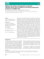
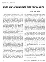
For example, the cycle in Figure 1(a) is given by
the path racing
1
n
→ contest
1
n

→ race
3
n
→ run
3
n
→
racing
1
n
in the WordNet dictionary graph. In fact
racing
1
n
contest
1
n
race
3
n
run
3
n
(a)
racing
1
n
contest
1
n

compete
1
v
race
2
v
(b)
Figure 1: An example of cycle (a) and quasi-cycle
(b) in WordNet.
contest
n
occurs in the gloss of racing
1
n
, race
3
n
is a
hyponym of contest
1
n
, and so on.
We further provide the definition of quasi-cycle
as a sequence of edges in which the reversal of
the orientation of a single edge creates a cycle
(Bohman and Thoma, 2000). For instance, the
quasi-cycle in Figure 1(b) is given by the path rac-
ing
1
n

→ contest
1
n
→ compete
1
v
→ race
2
v
← rac-
ing
1
n
. In fact, the reversal of the edge (racing
1
n
,
race
2
v
) creates a cycle.
Finally, we call a path a (quasi-)cycle if it is ei-
ther a cycle or a quasi-cycle. Further, we say that
a path is (quasi-)cyclic if it forms a (quasi-)cycle
in the graph.
2.2 The CQC Algorithm
Given a dictionary graph G = (V, E) built as de-
scribed in the previous section, our objective is
to disambiguate dictionary glosses with the sup-
port of (quasi-)cycles. (Quasi-)cyclic paths are in-

tuitively better than unconstrained paths as each
sense choice s is reinforced by the very fact of s
being reachable from itself through a sequence of
other senses.
Let a(s) be the set of ambiguous words to be
disambiguated in the part-of-speech tagged gloss
of sense s. Given a word w

∈ a(s), our aim is
to disambiguate w

according to the sense inven-
tory of D, i.e. to assign it the right sense chosen
from its set of senses Senses(w

). To this end, we
propose the use of a graph-based algorithm which
searches the dictionary graph and collects the fol-
lowing kinds of (quasi-)cyclic paths:
i) s → s

→ s
1
→ · · · → s
n−2
→ s (cycle)
ii) s → s

→ s
1

→ · · · → s
n−2
← s
(quasi-cycle)
595
CQC-Algorithm(s, w

)
1 for each sense s

∈ Senses(w

)
2 CQC(s

) := DFS(s

, s)
3 All CQC :=

s

∈Senses(w

)
CQC(s

)
4 for each sense s


∈ Senses(w

)
5 score(s

) := 0
6 for each path c ∈ CQC(s

)
7 l := length(c)
8 v := ω(l) ·
1
NumCQC(All CQC,l)
9 score(s

) := score(s

) + v
10 return argmax
s

∈Senses(w

)
score(s

)
Table 1: The Cycles and Quasi-Cycles (CQC) al-
gorithm in pseudocode.
where s is our source sense, s


is a candidate sense
of w

∈ gloss(s), s
i
is a sense in V , and n is
the length of the path (given by the number of its
edges). We note that both kinds of paths start and
end with the same vertex s, and that we restrict
quasi-cycles to those whose inverted edge departs
from s. To avoid any redundancy, we require that
no vertex is repeated in the path aside from the
start/end vertex (i.e. s = s

= s
i
= s
j
for any
i, j ∈ {1, . . . , n − 2}).
The Cycles and Quasi-Cycles (CQC) algorithm,
reported in pseudo-code in Table 1, takes as input a
source sense s and a target word w

(in our setting
2
w

∈ a(s)). It consists of two main phases.

During steps 1-3, cycles and quasi-cycles are
sought for each sense of w

. This step is per-
formed with a depth-first search (DFS, cf. (Cor-
men et al., 1990, pp. 477–479)) up to a depth
δ. To this end, we first define next(s) = {s

:
(s, s

) ∈ E}, that is the set of senses which can
be directly reached from sense s. The DFS starts
from a sense s

∈ Senses(w

), and recursively ex-
plores the senses in next(s

) until sense s or a
sense in next(s) is encountered, obtaining a cy-
cle or a quasi-cycle, respectively. For each sense
s

of w

the DFS returns the full set CQC(s

)

of (quasi-)cyclic paths collected. Note that the
DFS recursively keeps track of previously visited
senses, so as to discard (quasi-)cycles including
the same sense twice. Finally, in step 3, All
CQC
is set to store the cycles and quasi-cycles for all
the senses of w

.
2
Note that potentially w

can be any word of interest. The
very same algorithm can be applied to determine semantic
similarity or to disambiguate collocations.
The second phase (steps 4-10) computes a score
for each sense s

of w

based on the paths col-
lected for s

during the first phase. Let c be such
a path, and let l be its length, i.e. the number of
edges in the path. Then the contribution of c to the
score of s

is given by a function of its length ω(l),
which associates with l a number between 0 and 1.

This contribution is normalized by a factor given
by NumCQC(All CQC, l), which calculates the
overall number of paths of length l. In this work,
we will employ the function ω(l) = 1/e
l
, which
weighs a path with the inverse of the exponential
of its length (so as to exponentially decrease the
contribution of longer paths)
3
. Steps 4-9 are re-
peated for each candidate sense of w

. Finally, step
10 returns the highest-scoring sense of w

.
As a result of the systematic application of
the CQC algorithm to the dictionary graph G =
(V, E) associated with a dictionary D, a graph
ˆ
G = (V,
ˆ
E) is output, where V is again the sense
inventory of D, and
ˆ
E ⊆ E, such that each edge
(s, s

) ∈

ˆ
E either represents an unambiguous re-
lation in E (i.e. it was either a lexico-semantic re-
lation in D or a relation between s and a monose-
mous word occurring in its gloss) or is the result
of an execution of the CQC algorithm with input s
and w

∈ a(s).
2.3 An Example
Consider the following example: WordNet defines
the third sense of flesh
n
as “a soft moist part of a
fruit”. As a result of part-of-speech tagging, we
obtain:
gloss(flesh
3
n
) = {soft
a
, moist
a
, part
n
, fruit
n
}
Let us assume we aim to disambiguate the noun
fruit. Our call to the CQC algorithm in Table 1 is

then CQC-Algorithm(flesh
3
n
, fruit
n
).
As a result of the first two steps of the algorithm,
a set of cycles and quasi-cycles for each sense of
fruit
n
is collected, based on a DFS starting from
the respective senses of our target word (we as-
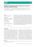
sume δ = 5). In Figure 2, we show some of the
(quasi-)cycles collected for senses #1 and #3 of
fruit
n
, respectively defined as “the ripened repro-
ductive body of a seed plant” and “an amount of
a product” (we neglect sense #2 as the length and
number of its paths is not dissimilar from that of
sense #3).
3
Other weight functions, such as ω(l) = 1 (which weighs
each path independent of its length) proved to perform worse.
596
flesh
3
n
fruit
1

n
berry1
1
n
pulpy
1
a
parenchyma
1
n
plant tissue
1
n
lychee
1
n
custard apple
1
n
mango
2
n
moist
1
a
flora
2
n
edible fruit
1

n
skin
2
n
hygrophyte
1
n
(a)
flesh
3
n
fruit
3
n
newspaper
4
n
mag
1
n
production
4
n
(b)
Figure 2: Some cycles and quasi-cycles connect-
ing flesh
3
n
to fruit
1

n
(a), and fruit
3
n
(b).
During the second phase of the algorithm, and
for each sense of fruit
n
, the contribution of each
(quasi-)cycle is calculated (steps 6-9 of the algo-
rithm). For example, for sense fruit
1
n
in Figure
2(a), 5 (quasi-)cycles of length 4 and 2 of length 5
were returned by DFS(fruit
1
n
, flesh
3
n
). As a result,
the following score is calculated:
4
score(fruit
1
n
) =
5
e

4
·
1
NumCQC(all chains,4)
+
2
e
5
·
1
NumCQC(all chains,5)
=
5
e
4
·7
+
2
e
5
·2
= 0.013 + 0.006 = 0.019
whereas for fruit
3
n
(see Figure 2(b)) we get:
score(fruit
3
n
) =

2
e
4
·
1
NumCQC(all chains,4)
=
2
e
4
·7
= 0.005
where NumCQC(All CQC, l) is the total num-
ber of cycles and quasi-cycles of length l over all
the senses of fruit
n
(according to Figure 2, this
amounts to 7 paths for l = 4 and 2 paths for l = 5).
Finally, the sense with the highest score (i.e.
fruit
1
n
) is returned.
3 Experiments
To test and compare the performance of our al-
gorithm, we performed a set of experiments on a
4
Note that, for the sake of simplicity, we are calculating
our scores based on the paths shown in Figure 2. However,
we tried to respect the proportion of paths collected by the

algorithm for the two senses.
variety of resources. First, we summarize the re-
sources (Section 3.1) and algorithms (Section 3.2)
that we adopted. In Section 3.3 we report our ex-
perimental results.
3.1 Resources
The following resources were used in our experi-
ments:
• WordNet (Fellbaum, 1998), the most
widespread computational lexicon of En-
glish. It encodes concepts as synsets, and
provides textual glosses and lexico-semantic
relations between synsets. Its latest version
(3.0) contains around 155,000 lemmas, and
over 200,000 word senses;
• Macquarie Concise Dictionary (Yallop,
2006), a machine-readable dictionary of
(Australian) English, which includes around
50,000 lemmas and almost 120,000 word
senses, for which it provides textual glosses
and examples;
• Ragazzini/Biagi Concise (Ragazzini and Bi-
agi, 2006), a bilingual English-Italian dic-
tionary, containing over 90,000 lemmas and
150,000 word senses. The dictionary pro-
vides Italian translations for each English
word sense, and vice versa.
We used TreeTagger (Schmid, 1997) to part-of-
speech tag the glosses in the three resources.
3.2 Algorithms

Hereafter we briefly summarize the algorithms
that we applied in our experiments:
• CQC: we applied the CQC algorithm as de-
scribed in Section 2.2;
• Cycles, which applies the CQC algorithm but
searches for cycles only (i.e. quasi-cycles are
not collected);
• An adaptation of the Lesk algorithm (Lesk,
1986), which, given a source sense s of word
w and a word w

occurring in the gloss of s,
determines the right sense of w

as that which
maximizes the (normalized) overlap between
each sense s

of w

and s:
argmax
s

∈Senses(w

)
|next
∗
(s) ∩ next

∗
(s

)|
max{|next
∗
(s)|, |next
∗
(s

)|}
597
where we define next
∗
(s) = words(s) ∪
next(s), and words(s) is the set of lexical-
izations of sense s (e.g. the synonyms in the
synset s). When WordNet is our reference re-
source, we employ an extension of the Lesk
algorithm, namely Extended Gloss Overlap
(Banerjee and Pedersen, 2003), which ex-
tends the sense definition with words from
the definitions of related senses (such as hy-
pernyms, hyponyms, etc.). We use the same
set of relations available in the authors’ im-
plementation of the algorithm.
We also compared the performance of the above
algorithms with two standard baselines, namely
the First Sense Baseline (abbreviated as FS BL)
and the Random Baseline (Random BL).

3.3 Results
Our experiments concerned the disambiguation of
the gloss words in three datasets, one for each re-
source, namely WordNet, Macquarie Concise, and
Ragazzini/Biagi. In all datasets, given a sense s,
our set a(s) is given by the set of part-of-speech-
tagged ambiguous content words in the gloss of
sense s from our reference dictionary.
WordNet. When using WordNet as a reference
resource, given a sense s whose gloss we aim to
disambiguate, the dictionary graph includes not
only edges connecting s to senses of gloss words
(step (iii) of the graph construction procedure, cf.
Section 2.1), but also those obtained from any of
the WordNet lexico-semantics relations (step (ii)).
For WordNet gloss disambiguation, we em-
ployed the dataset used in the Senseval-3 Gloss
WSD task (Litkowski, 2004), which contains
15,179 content words from 9,257 glosses
5
. We
compared the performance of CQC, Cycles, Lesk,
and the two baselines. To get full coverage and
high performance, we learned a threshold for each
system below which they recur to the FS heuris-
tic. The threshold and maximum path length were
tuned on a small in-house manually-annotated
dataset of 100 glosses. The results are shown in
Table 2. We also included in the table the perfor-
mance of the best-ranking system in the Senseval-

5
Recently, Princeton University released a richer corpus
of disambiguated glosses, namely the “Princeton WordNet
Gloss Corpus” ().
However, in order to allow for a comparison with the state
of the art (see below), we decided to adopt the Senseval-3
dataset.
Algorithm Prec./Recall
CQC 64.25
Cycles 63.74
Lesk 51.75
TALP 68.60/68.30
FS BL 55.44
Random BL 26.29
Table 2: Gloss WSD performance on WordNet.
3 Gloss WSD task, namely the TALP system
(Castillo et al., 2004).
CQC outperforms all other proposed ap-
proaches, obtaining a 64.25% precision and recall.
We note that Cycles also gets high performance,
compared to Lesk and the baselines. Also, com-
pared to CQC, the difference is not statistically
significant. However, we observe that, if we do
not recur to the first sense as a backoff strategy, we
get a much lower recall for Cycles (P = 65.39, R =
26.70 for CQC, P = 72.03, R = 16.39 for Cycles).
CQC performs about 4 points below the TALP
system. As also discussed later, we believe this re-
sult is relevant, given that our approach does not
rely on additional knowledge resources, as TALP

does (though both algorithms recur to the FS back-
off strategy).
Finally, we observe that the FS baseline has
lower performance than in typical all-words dis-
ambiguation settings (usually above 60% accu-
racy). We believe that this is due to the absence
of monosemous words from the test set, and to
the possibly different distribution of senses in the
dataset.
Macquarie Concise. Automatically disam-
biguating glosses in a computational lexicon
such as WordNet is certainly useful. However,
disambiguating a machine-readable dictionary
is an even more ambitious task. In fact, while
computational lexicons typically encode some ex-
plicit semantic relations which can be used as an
aid to the disambiguation task, machine-readable
dictionaries only rarely provide sense-tagged
information (often in the form of references to
other word senses). As a result, in this latter
setting the dictionary graph typically contains
only edges obtained from the gloss words of sense
s (step (iii), Section 2.1).
To experiment with machine-readable dictio-
naries, we employed the Macquarie Concise Dic-
598
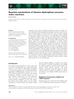
Algorithm Prec./Recall
CQC 77.13
Cycles 67.63
Lesk 30.16

FS BL 51.48
Random BL 23.28
Table 3: Gloss WSD performance on Macquarie
Concise.
tionary (Yallop, 2006). A dataset was prepared
by randomly selecting 1,000 word senses from
the dictionary and annotating the content words in
their glosses according to the dictionary sense in-
ventory. Overall, 2,678 words were sense tagged.
The results are shown in Table 3. CQC obtains
an accuracy of 77.13% (in case of ties, a random
choice is made, thus leading to the same precision
and recall), Cycles achieves an accuracy of almost
10% less than CQC (the difference is statistically
significant; p < 0.01). The FS baseline, here, is
based on the first sense listed in the Macquarie
sense inventory, which – in contrast to WordNet
– does not depend on the occurrence frequency of
senses in a semantically-annotated corpus. How-
ever, we note that the FS baseline is not very dif-
ferent from that of the WordNet experiment.
We observe that the Lesk performance is very
low on this dataset (around 7 points above the Ran-
dom BL), due to the impossibility of using the
Extended Gloss Overlap approach (semantic rela-
tions are not available in the Macquarie Concise)
and to the low number of matches between source
and target entries.
Ragazzini/Biagi. Finally, we performed an ex-
periment on the Ragazzini/Biagi English-Italian

machine-readable dictionary. In this experiment,
disambiguating a word w

in the gloss of a sense
s from one section (e.g. Italian-English) equals to
selecting a word sense s

of w

listed in the other
section of the dictionary (e.g. English-Italian). For
example, given the English entry race
1
n
, translated
as “corsa
n
, gara
n
”, our objective is to assign the
right Italian sense from the Italian-English section
to corsa
n
and gara
n
.
To apply the CQC algorithm, a simple adapta-
tion is needed, so as to allow (quasi-)cycles to con-
nect word senses from the two distinct sections.
The algorithm must seek cyclic and quasi-cyclic

paths, respectively of the kind:
Algorithm Prec./Recall
CQC 89.34
Cycles 85.40
Lesk 63.89
FS BL 73.15
Random BL 51.69
Table 4: Gloss WSD performance on Ragazz-
ini/Biagi.
i) s → s

→ s
1
→ · · · → s
n−2
→ s
ii) s → s

→ s
1
→ · · · → s
n−2
← s
where n is the path length, s and s

are senses re-
spectively from the source (e.g. Italian/English)
and the target (e.g. English/Italian) section of the
dictionary, s
i

is a sense from the target section for
i ≤ k and from the source section for i > k,
for some k such that 0 ≤ k ≤ n − 2. In other
words, the DFS can jump at any time from the tar-
get section to the source section. After the jump,
the depth search continues in the source section, in
the hope to reach s. For example, the following is
a cycle with k = 1:
race
1
n
→ corsa
2
n
→ gara
2
n
→ race
1
n
where the edge between corsa
2
n
and gara
2
n
is due
to the occurrence of gara
n
in the gloss of corsa

2
n
as a domain label for that sense.
To perform this experiment, we randomly se-
lected 250 entries from each section (500 over-
all), including a total number of 1,069 translations
that we manually sense tagged. In Table 4 we re-
port the results of CQC, Cycles and Lesk on this
task. Overall, the figures are higher than in previ-
ous experiments, thanks to a lower average degree
of polysemy of the resource, which also impacts
positively on the FS baseline. However, given a
random baseline of 51.69%, the performance of
CQC, over 89% precision and recall, is signif-
icantly higher. Cycles obtains around 4 points
less than CQC (the difference is statistically sig-
nificant; p < 0.01). The performance of Lesk
(63.89%) is also much higher than in our previ-
ous experiments, thanks to the higher chance of
finding a 1:1 correspondence between the two sec-
tions. However, we observed that this does not al-
ways hold, as also supported by the better results
of CQC.
599
4 Discussion
The experiments presented in the previous section
are inherently heterogeneous, due to the different
nature of the resources adopted (a computational
lexicon, a monolingual and a bilingual machine-
readable dictionary). Our aim was to show the

flexibility of our approach in tagging gloss words
with senses from the same dictionary.
We show the average polysemy of the three
datasets in Table 5. Notice that none of the
datasets included monosemous items, so our ex-
periments cannot be compared to typical all-words
disambiguation tasks, where monosemous words
are part of the test set.
Given that words in the Macquarie dataset have
a higher average polysemy than in the Word-
Net dataset, one might wonder why disambiguat-
ing glosses from a computational lexicon such as
WordNet is more difficult than performing a sim-
ilar task on a machine-readable dictionary such
as the Macquarie Concise Dictionary, which does
not provide any explicit semantic hint. We be-
lieve there are at least two reasons for this out-
come: the first specifically concerns the Senseval-
3 Gloss WSD dataset, which does not reflect the
distribution of genus-differentiae terms in dictio-
nary glosses: less than 10% of the items were hy-
pernyms, thus making the task harder. As for the
second reason, we believe that the Macquarie Con-
cise provides more clear-cut definitions, thus mak-
ing sense assignments relatively easier.
An analytical comparison of the results of Cy-
cles and CQC show that, especially for machine-
readable dictionaries, employing both cycles and
quasi-cycles is highly beneficial, as additional sup-
port is provided by the latter patterns. Our results

on WordNet prove to be more difficult to analyze,
because of the need of employing the first sense
heuristic to get full coverage. Also, the maximum
path length used for WordNet was different (δ = 3
according to our tuning, compared to δ = 4 for
Macquarie and Ragazzini/Biagi). However, quasi-
cycles are shown to provide over 10% improve-
ment in terms of recall (at the price of a decrease
in precision of 6.6 points).
Further, we note that the performance of the
CQC algorithm dramatically improves as the max-
imum score (i.e. the score which leads to a sense
assignment) increases. As a result, users can tune
the disambiguation performance based on their
specific needs (coverage, precision, etc.). For in-
WN Mac R/B
Polysemy 6.68 7.97 3.16
Table 5: Average polysemy of the three datasets.
stance, WordNet Gloss WSD can perform up to
85.7% precision and 10.1% recall if we require the
score to be ≥ 0.2 and do not use the FS baseline as
a backoff strategy. Similarly, we can reach up to
93.8% prec., 20.0% recall for Macquarie Concise
(score ≥ 0.12) and even 95.2% prec., 70.6% recall
(score ≥ 0.1) for Ragazzini/Biagi.
5 Related Work
Word Sense Disambiguation is a large research
field (see (Navigli, 2009) for an up-to-date
overview). However, in this paper we focused on
a specific kind of WSD, namely the disambigua-

tion of dictionary definitions. Seminal works on
the topic date back to the late 1970s, with the de-
velopment of models for the identification of tax-
onomies from lexical resources (Litkowski, 1978;
Amsler, 1980). Subsequent works focused on the
identification of genus terms (Chodorow et al.,
1985) and, more in general, on the extraction of
explicit information from machine-readable dic-
tionaries (see, e.g., (Nakamura and Nagao, 1988;
Ide and V
´
eronis, 1993)). Kozima and Furugori
(1993) provide an approach to the construction
of ambiguous semantic networks from glosses in
the Longman Dictionary of Contemporary English
(LDOCE). In this direction, it is worth citing the
work of Vanderwende (1996) and Richardson et
al. (1998), who describe the construction of Mind-
Net, a lexical knowledge base obtained from the
automated extraction of lexico-semantic informa-
tion from two machine-readable dictionaries. As a
result, weighted relation paths are produced to in-
fer the semantic similarity between pairs of words.
Several heuristics have been presented for the
disambiguation of the genus of a dictionary defini-
tion (Wilks et al., 1996; Rigau et al., 1997). More
recently, a set of heuristic techniques has been pro-
posed to semantically annotate WordNet glosses,
leading to the release of the eXtended WordNet
(Harabagiu et al., 1999; Moldovan and Novischi,

2004). Among the methods, the cross reference
heuristic is the closest technique to our notion of
cycles and quasi-cycles. Given a pair of words w
and w

, this heuristic is based on the occurrence of
600
w in the gloss of a sense s

of w

and, vice versa,
of w

in the gloss of a sense s of w. In other words,
a graph cycle s → s

→ s of length 2 is sought.
Based on the eXtended WordNet, a gloss dis-
ambiguation task was organized at Senseval-3
(Litkowski, 2004). Interestingly, the best perform-
ing systems, namely the TALP system (Castillo et
al., 2004), and SSI (Navigli and Velardi, 2005),
are knowledge-based and rely on rich knowledge
resources: respectively, the Multilingual Central
Repository (Atserias et al., 2004), and a propri-
etary lexical knowledge base.
In contrast, the approach presented in this paper
performs the disambiguation of ambiguous words
by exploiting only the reference dictionary itself.

Furthermore, as we showed in Section 3.3, our
method does not rely on WordNet, and can be ap-
plied to any lexical knowledge resource, including
bilingual dictionaries.
Finally, methods in the literature more focused
on a specific disambiguation task include statisti-
cal methods for the attachment of hyponyms un-
der the most likely hypernym in the WordNet tax-
onomy (Snow et al., 2006), structural approaches
based on semantic clusters and distance met-
rics (Pennacchiotti and Pantel, 2006), supervised
machine learning methods for the disambiguation
of meronymy relations (Girju et al., 2003), etc.
6 Conclusions
In this paper we presented a novel approach to dis-
ambiguate the glosses of computational lexicons
and machine-readable dictionaries, with the aim of
alleviating the knowledge acquisition bottleneck.
The method is based on the identification of cy-
cles and quasi-cycles, i.e. circular edge sequences
(possibly with one edge reversed) relating a source
to a target word sense.
The strength of the approach lies in its weakly
supervised nature: (quasi-)cycles rely exclusively
on the structure of the input lexical resources. No
additional resource (such as labeled corpora or ex-
ternal knowledge bases) is required, assuming we
do not resort to the FS baseline. As a result, the
approach can be applied to obtain a semantic net-
work from the disambiguation of virtually any lex-

ical resource available in machine-readable format
for which a sense inventory is provided.
The utility of gloss disambiguation is even
greater in bilingual dictionaries, as idiosyncrasies
such as missing or redundant translations can be
discovered, thus helping lexicographers improve
the resources
6
. An adaptation similar to that de-
scribed for disambiguating the Ragazzini/Biagi
can be employed for mapping pairs of lexical
resources (e.g. FrameNet (Baker et al., 1998)
to WordNet), thus contributing to the beneficial
knowledge integration process. Following this di-
rection, we are planning to further experiment on
the mapping of FrameNet, VerbNet (Kipper et al.,
2000), and other lexical resources.
The graphs output by the CQC algo-
rithm for our datasets are available from
We
are scheduling the release of a software pack-
age which includes our implementation of the
CQC algorithm and allows its application to any
resource for which a standard interface can be
written.
Finally, starting from the work of Budanitsky
and Hirst (2006), we plan to experiment with the
CQC algorithm when employed as a semantic sim-
ilarity measure, and compare it with the most suc-
cessful existing approaches. Although in this pa-

per we focused on the disambiguation of dictio-
nary glosses, the same approach can be applied for
disambiguating collocations according to a dictio-
nary of choice, thus providing a way to further en-
rich lexical resources with external knowledge.
Acknowledgments
The author is grateful to Ken Litkowski and the
anonymous reviewers for their useful comments.
He also wishes to thank Zanichelli and Macquarie
for kindly making their dictionaries available for
research purposes.
References
Robert A. Amsler. 1980. The structure of the
Merriam-Webster pocket dictionary, Ph.D. Thesis.
University of Texas, Austin, TX, USA.
Jordi Atserias, Lu
´
ıs Villarejo, German Rigau, Eneko
Agirre, John Carroll, Bernardo Magnini, and Piek
Vossen. 2004. The meaning multilingual central
repository. In Proceedings of GWC 2004, pages 23–
30, Brno, Czech Republic.
Collin F. Baker, Charles J. Fillmore, and John B. Lowe.
1998. The berkeley framenet project. In Proceed-
ings of COLING-ACL 1998, pages 86–90, Montreal,
Canada.
6
This is indeed an ongoing line of research in collabora-
tion with the Zanichelli dictionary publisher.
601

Satanjeev Banerjee and Ted Pedersen. 2003. Extended
gloss overlaps as a measure of semantic relatedness.
In Proceedings of IJCAI 2003, pages 805–810, Aca-
pulco, Mexico.
John Bernard, editor. 1986. Macquarie Thesaurus.
Macquarie, Sydney, Australia.
Tom Bohman and Lubos Thoma. 2000. A note on
sparse random graphs and cover graphs. The Elec-
tronic Journal of Combinatorics, 7:1–9.
Alexander Budanitsky and Graeme Hirst. 2006. Eval-
uating wordnet-based measures of semantic dis-
tance. Computational Linguistics, 32(1):13–47.
Mauro Castillo, Francis Real, Jordi Asterias, and Ger-
man Rigau. 2004. The talp systems for dis-
ambiguating wordnet glosses. In Proceedings of
ACL 2004 SENSEVAL-3 Workshop, pages 93–96,
Barcelona, Spain.
Martin Chodorow, Roy Byrd, and George Heidorn.
1985. Extracting semantic hierarchies from a large
on-line dictionary. In Proceedings of ACL 1985,
pages 299–304, Chicago, IL, USA.
Thomas H. Cormen, Charles E. Leiserson, and
Ronald L. Rivest. 1990. Introduction to algorithms.
MIT Press, Cambridge, MA.
Montse Cuadros and German Rigau. 2006. Quality
assessment of large scale knowledge resources. In
Proceedings of EMNLP 2006, pages 534–541, Syd-
ney, Australia.
Philip Edmonds. 2000. Designing a task for
SENSEVAL-2. Technical note.

Christiane Fellbaum, editor. 1998. WordNet: An Elec-
tronic Database. MIT Press, Cambridge, MA.
Roxana Girju, Adriana Badulescu, and Dan Moldovan.
2003. Learning semantic constraints for the auto-
matic discovery of part-whole relations. In Proceed-
ings of NAACL 2003, pages 1–8, Edmonton, Canada.
Sanda Harabagiu, George Miller, and Dan Moldovan.
1999. Wordnet 2 - a morphologically and se-
mantically enhanced resource. In Proceedings of
SIGLEX-99, pages 1–8, Maryland, USA.
Nancy Ide and Jean V
´
eronis. 1993. Extracting
knowledge bases from machine-readable dictionar-
ies: Have we wasted our time? In Proceedings
of Workshop on Knowledge Bases and Knowledge
Structures, pages 257–266, Tokyo, Japan.
Karin Kipper, Hoa Trang Dang, and Martha Palmer.
2000. Class-based construction of a verb lexicon. In
Proceedings of AAAI 2000, pages 691–696, Austin,
TX, USA.
Hideki Kozima and Teiji Furugori. 1993. Similarity
between words computed by spreading activation on
an english dictionary. In Proceedings of ACL 1993,
pages 232–239, Utrecht, The Netherlands.
Michael Lesk. 1986. Automatic sense disambiguation
using machine readable dictionaries: How to tell a
pine cone from an ice cream cone. In Proceedings
of the 5
th

SIGDOC, pages 24–26, New York, NY.
Kenneth C. Litkowski. 1978. Models of the semantic
structure of dictionaries. American Journal of Com-
putational Linguistics, (81):25–74.
Kenneth C. Litkowski. 2004. Senseval-3 task:
Word-sense disambiguation of wordnet glosses. In
Proceedings of ACL 2004 SENSEVAL-3 Workshop,
pages 13–16, Barcelona, Spain.
Dan Moldovan and Adrian Novischi. 2004. Word
sense disambiguation of wordnet glosses. Computer
Speech & Language, 18:301–317.
Jun-Ichi Nakamura and Makoto Nagao. 1988. Extrac-
tion of semantic information from an ordinary en-
glish dictionary and its evaluation. In Proceedings
of COLING 1988, pages 459–464, Budapest, Hun-
gary.
Roberto Navigli and Paola Velardi. 2005. Structural
semantic interconnections: a knowledge-based ap-
proach to word sense disambiguation. IEEE Trans-
actions of Pattern Analysis and Machine Intelligence
(TPAMI), 27(7):1075–1088.
Roberto Navigli. 2009. Word sense disambiguation: a
survey. ACM Computing Surveys, 41(2):1–69.
Marco Pennacchiotti and Patrick Pantel. 2006. On-
tologizing semantic relations. In Proceedings of
COLING-ACL 2006, pages 793–800, Sydney, Aus-
tralia.
Paul Proctor, editor. 1978. Longman Dictionary of
Contemporary English. Longman Group, UK.
Giuseppe Ragazzini and Adele Biagi, editors. 2006. Il

Ragazzini-Biagi, 4
th
Edition. Zanichelli, Italy.
Stephen D. Richardson, William B. Dolan, and Lucy
Vanderwende. 1998. Mindnet: acquiring and struc-
turing semantic information from text. In Proceed-
ings of COLING 1998, pages 1098–1102, Montreal,
Quebec, Canada.
German Rigau, Jordi Atserias, and Eneko Agirre.
1997. Combining unsupervised lexical knowledge
methods for word sense disambiguation. In Pro-
ceedings of ACL/EACL 1997, pages 48–55, Madrid,
Spain.
Peter M. Roget. 1911. Roget’s International The-
saurus (1
st
edition). Cromwell, New York, USA.
Helmut Schmid. 1997. Probabilistic part-of-speech
tagging using decision trees. In Daniel Jones and
Harold Somers, editors, New Methods in Language
Processing, Studies in Computational Linguistics,
pages 154–164. UCL Press, London, UK.
Rion Snow, Daniel Jurafsky, and Andrew Y. Ng. 2006.
Semantic taxonomy induction from heterogenous
evidence. In Proceedings of COLING-ACL 2006,
pages 801–808, Sydney, Australia.
Lucy Vanderwende. 1996. The analysis of noun se-
quences using semantic information extracted from
on-line dictionaries, Ph.D. Thesis. Georgetown
University, Washington, USA.

Yorick Wilks, Brian Slator, and Louise Guthrie, editors.
1996. Electric words: Dictionaries, computers and
meanings. MIT Press, Cambridge, MA.
Colin Yallop, editor. 2006. The Macquarie Concise
Dictionary 4
th
Edition. Macquarie Library Pty Ltd,
Sydney, Australia.
602