Báo cáo khoa học: "Paraphrase Identification as Probabilistic Quasi-Synchronous Recognition" ppt

Proceedings of the 47th Annual Meeting of the ACL and the 4th IJCNLP of the AFNLP, pages 468–476,
Suntec, Singapore, 2-7 August 2009.
c
2009 ACL and AFNLP
Paraphrase Identification as Probabilistic Quasi-Synchronous Recognition
Dipanjan Das and Noah A. Smith
Language Technologies Institute
Carnegie Mellon University
Pittsburgh, PA 15213, USA
{dipanjan,nasmith}@cs.cmu.edu
Abstract
We present a novel approach to decid-
ing whether two sentences hold a para-
phrase relationship. We employ a gen-
erative model that generates a paraphrase
of a given sentence, and we use proba-
bilistic inference to reason about whether
two sentences share the paraphrase rela-
tionship. The model cleanly incorporates
both syntax and lexical semantics using
quasi-synchronous dependency grammars
(Smith and Eisner, 2006). Furthermore,
using a product of experts (Hinton, 2002),
we combine the model with a comple-
mentary logistic regression model based
on state-of-the-art lexical overlap features.
We evaluate our models on the task of
distinguishing true paraphrase pairs from
false ones on a standard corpus, giving
competitive state-of-the-art performance.
1 Introduction

The problem of modeling paraphrase relation-
ships between natural language utterances (McK-
eown, 1979) has recently attracted interest. For
computational linguists, solving this problem may
shed light on how best to model the semantics
of sentences. For natural language engineers, the
problem bears on information management sys-
tems like abstractive summarizers that must mea-
sure semantic overlap between sentences (Barzi-
lay and Lee, 2003), question answering modules
(Marsi and Krahmer, 2005) and machine transla-
tion (Callison-Burch et al., 2006).
The paraphrase identification problem asks
whether two sentences have essentially the same
meaning. Although paraphrase identification is
defined in semantic terms, it is usually solved us-
ing statistical classifiers based on shallow lexical,
n-gram, and syntactic “overlap” features. Such
overlap features give the best-published classifi-
cation accuracy for the paraphrase identification
task (Zhang and Patrick, 2005; Finch et al., 2005;
Wan et al., 2006; Corley and Mihalcea, 2005, in-
ter alia), but do not explicitly model correspon-
dence structure (or “alignment”) between the parts
of two sentences. In this paper, we adopt a model
that posits correspondence between the words in
the two sentences, defining it in loose syntactic
terms: if two sentences are paraphrases, we expect
their dependency trees to align closely, though
some divergences are also expected, with some

more likely than others. Following Smith and Eis-
ner (2006), we adopt the view that the syntactic
structure of sentences paraphrasing some sentence
s should be “inspired” by the structure of s.
Because dependency syntax is still only a crude
approximation to semantic structure, we augment
the model with a lexical semantics component,
based on WordNet (Miller, 1995), that models how
words are probabilistically altered in generating
a paraphrase. This combination of loose syntax
and lexical semantics is similar to the “Jeopardy”
model of Wang et al. (2007).
This syntactic framework represents a major de-
parture from useful and popular surface similarity
features, and the latter are difficult to incorporate
into our probabilistic model. We use a product of
experts (Hinton, 2002) to bring together a logis-
tic regression classifier built from n-gram overlap
features and our syntactic model. This combined
model leverages complementary strengths of the
two approaches, outperforming a strong state-of-
the-art baseline (Wan et al., 2006).
This paper is organized as follows. We intro-
duce our probabilistic model in §2. The model
makes use of three quasi-synchronous grammar
models (Smith and Eisner, 2006, QG, hereafter) as
components (one modeling paraphrase, one mod-
eling not-paraphrase, and one a base grammar);
these are detailed, along with latent-variable in-
ference and discriminative training algorithms, in

§3. We discuss the Microsoft Research Paraphrase
Corpus, upon which we conduct experiments, in
§4. In §5, we present experiments on paraphrase
468
identification with our model and make compar-
isons with the existing state-of-the-art. We de-
scribe the product of experts and our lexical over-
lap model, and discuss the results achieved in §6.
We relate our approach to prior work (§7) and con-
clude (§8).
2 Probabilistic Model
Since our task is a classification problem, we re-
quire our model to provide an estimate of the pos-
terior probability of the relationship (i.e., “para-
phrase,” denoted p, or “not paraphrase,” denoted
n), given the pair of sentences.
1
Here, p
Q
denotes
model probabilities, c is a relationship class (p or
n), and s
1
and s
2
are the two sentences. We choose
the class according to:
ˆc = argmax
c∈{p,n}
p

Q
(c | s
1
, s
2
)
= argmax
c∈{p,n}
p
Q
(c) × p
Q
(s
1
, s
2
| c) (1)
We define the class-conditional probabilities of
the two sentences using the following generative
story. First, grammar G
0
generates a sentence s.
Then a class c is chosen, corresponding to a class-
specific probabilistic quasi-synchronous grammar
G
c
. (We will discuss QG in detail in §3. For the
present, consider it a specially-defined probabilis-
tic model that generates sentences with a specific
property, like “paraphrases s,” when c = p.) Given

s, G
c
generates the other sentence in the pair, s

.
When we observe a pair of sentences s
1
and s
2
we do not presume to know which came first (i.e.,
which was s and which was s

). Both orderings
are assumed to be equally probable. For class c,
p
Q
(s
1
, s
2
| c) =
0.5 × p
Q
(s
1
| G
0
) × p
Q
(s

2
| G
c
(s
1
))
+ 0.5 × p
Q
(s
2
| G
0
) × p
Q
(s
1
| G
c
(s
2
))(2)
where c can be p or n; G
p
(s) is the QG that gen-
erates paraphrases for sentence s, while G
n
(s) is
the QG that generates sentences that are not para-
phrases of sentence s. This latter model may seem
counter-intuitive: since the vast majority of pos-

sible sentences are not paraphrases of s, why is a
special grammar required? Our use of a G
n
fol-
lows from the properties of the corpus currently
used for learning, in which the negative examples
1
Although we do not explore the idea here, the model
could be adapted for other sentence-pair relationships like en-
tailment or contradiction.
were selected to have high lexical overlap. We re-
turn to this point in §4.
3 QG for Paraphrase Modeling
Here, we turn to the models G
p
and G
n
in detail.
3.1 Background
Smith and Eisner (2006) introduced the quasi-
synchronous grammar formalism. Here, we de-
scribe some of its salient aspects. The model
arose out of the empirical observation that trans-
lated sentences have some isomorphic syntactic
structure, but divergences are possible. Therefore,
rather than an isomorphic structure over a pair of
source and target sentences, the syntactic tree over
a target sentence is modeled by a source sentence-
specific grammar “inspired” by the source sen-
tence’s tree. This is implemented by associating

with each node in the target tree a subset of the
nodes in the source tree. Since it loosely links
the two sentences’ syntactic structures, QG is well
suited for problems like word alignment for MT
(Smith and Eisner, 2006) and question answering
(Wang et al., 2007).
Consider a very simple quasi-synchronous
context-free dependency grammar that generates
one dependent per production rule.
2
Let s =
s
1
, , s
m
 be the source sentence. The grammar
rules will take one of the two forms:
t, l → t, lt

, k or t, l → t

, kt, l
where t and t

range over the vocabulary of the
target language, and l and k ∈ {0, , m} are in-
dices in the source sentence, with 0 denoting null.
3
Hard or soft constraints can be applied between l
and k in a rule. These constraints imply permissi-

ble “configurations.” For example, requiring l = 0
and, if k = 0 then s
k
must be a child of s
l
in the
source tree, we can implement a synchronous de-
pendency grammar similar to (Melamed, 2004).
Smith and Eisner (2006) used a quasi-
synchronous grammar to discover the correspon-
dence between words implied by the correspon-
dence between the trees. We follow Wang et al.
(2007) in treating the correspondences as latent
variables, and in using a WordNet-based lexical
semantics model to generate the target words.
2
Our actual model is more complicated; see §3.2.
3
A more general QG could allow one-to-many align-
ments, replacing l and k with sets of indices.
469
3.2 Detailed Model
We describe how we model p
Q
(t | G
p
(s)) and
p
Q
(t | G

n
(s)) for source and target sentences s
and t (appearing in Eq. 2 alternately as s
1
and s
2
).
A dependency tree on a sequence w =
w
1
, , w
k
 is a mapping of indices of words to
indices of syntactic parents, τ
p
: {1, , k} →
{0, , k}, and a mapping of indices of words to
dependency relation types in L, τ

: {1, , k} →
L. The set of indices children of w
i
to its left,
{j : τ
w
(j) = i, j < i}, is denoted λ
w
(i), and
ρ
w

(i) is used for right children. w
i
has a single
parent, denoted by w
τ
p
(i)
. Cycles are not allowed,
and w
0
is taken to be the dummy “wall” symbol,
$, whose only child is the root word of the sen-
tence (normally the main verb). The label for w
i
is denoted by τ

(i). We denote the whole tree of
a sentence w by τ
w
, the subtree rooted at the ith
word by τ
w,i
.
Consider two sentences: let the source sen-
tence s contain m words and the target sentence
t contain n words. Let the correspondence x :
{1, , n} → {0, , m} be a mapping from in-
dices of words in t to indices of words in s. (We
require each target word to map to at most one
source word, though multiple target words can

map to the same source word, i.e., x(i) = x(j)
while i = j.) When x(i) = 0, the ith target word
maps to the wall symbol, equivalently a “null”
word. Each of our QGs G
p
and G
n
generates the
alignments x, the target tree τ
t
, and the sentence
t. Both G
p
and G
n
are structured in the same way,
differing only in their parameters; henceforth we
discuss G
p
; G
n
is similar.
We assume that the parse trees of s and t are
known.
4
Therefore our model defines:
p
Q
(t | G
p

(s)) = p(τ
t
| G
p
(τ
s
))
=

x
p(τ
t
, x | G
p
(τ
s
)) (3)
Because the QG is essentially a context-free de-
pendency grammar, we can factor it into recur-
sive steps as follows (let i be an arbitrary index
in {1, , n}):
P (τ
t,i
| t
i
, x(i), τ
s
) = p
val
(|λ

t
(i)|, |ρ
t
(i)| | t
i
)
4
In our experiments, we use the parser described by Mc-
Donald et al. (2005), trained on sections 2–21 of the WSJ
Penn Treebank, transformed to dependency trees following
Yamada and Matsumoto (2003). (The same treebank data
were also to estimate many of the parameters of our model, as
discussed in the text.) Though it leads to a partial “pipeline”
approximation of the posterior probability p(c | s, t), we be-
lieve that the relatively high quality of English dependency
parsing makes this approximation reasonable.
×

j∈λ
t
(i)∪ρ
t
(i)
m

x(j)=0
P (τ
t,j
| t
j

, x(j), τ
s
)
×p
kid
(t
j
, τ
t

(j), x(j) | t
i
, x(i), τ
s
) (4)
where p
val
and p
kid
are valence and child-
production probabilities parameterized as dis-
cussed in §3.4. Note the recursion in the second-
to-last line.
We next describe a dynamic programming so-
lution for calculating p(τ
t
| G
p
(τ
s

)). In §3.4 we
discuss the parameterization of the model.
3.3 Dynamic Programming
Let C(i, l) refer to the probability of τ
t,i
, assum-
ing that the parent of t
i
, t
τ
t
p
(i)
, is aligned to s
l
. For
leaves of τ
t
, the base case is:
C(i, l) = p
val
(0, 0 | t
i
) × (5)

m
k=0
p
kid
(t

i
, τ
t

(i), k | t
τ
t
p
(i)
, l, τ
s
)
where k ranges over possible values of x(i), the
source-tree node to which t
i
is aligned. The recur-
sive case is:
C(i, l) = p
val
(|λ
t
(i)|, |ρ
t
(i)| | t
i
) (6)
×

m
k=0

p
kid
(t
i
, τ
t

(i), k | t
τ
t
p
(i)
, l, τ
s
)
×

j∈λ
t
(i)∪ρ
t
(i)
C(j, k)
We assume that the wall symbols t
0
and s
0
are
aligned, so p(τ
t

| G
p
(τ
s
)) = C(r, 0), where r is
the index of the root word of the target tree τ
t
. It
is straightforward to show that this algorithm re-
quires O(m
2
n) runtime and O(mn) space.
3.4 Parameterization
The valency distribution p
val
in Eq. 4 is estimated
in our model using the transformed treebank (see
footnote 4). For unobserved cases, the conditional
probability is estimated by backing off to the par-
ent POS tag and child direction.
We discuss next how to parameterize the prob-
ability p
kid
that appears in Equations 4, 5, and 6.
This conditional distribution forms the core of our
QGs, and we deviate from earlier research using
QGs in defining p
kid
in a fully generative way.
In addition to assuming that dependency parse

trees for s and t are observable, we also assume
each word w
i
comes with POS and named entity
tags. In our experiments these were obtained au-
tomatically using MXPOST (Ratnaparkhi, 1996)
and BBN’s Identifinder (Bikel et al., 1999).
470
For clarity, let j = τ
t
p
(i) and let l = x(j).
p
kid
(t
i
, τ
t

(i), x(i) | t
j
, l, τ
s
) =
p
config
(config(t
i
, t
j

, s
x(i)
, s
l
) | t
j
, l, τ
s
) (7)
×p
unif
(x(i) | config(t
i
, t
j
, s
x(i)
, s
l
)) (8)
×p
lab
(τ
t

(i) | config(t
i
, t
j
, s

x(i)
, s
l
)) (9)
×p
pos
(pos(t
i
) | pos(s
x(i)
)) (10)
×p
ne
(ne(t
i
) | ne(s
x(i)
)) (11)
×p
lsrel
(lsrel(t
i
) | s
x(i)
) (12)
×p
word
(t
i
| lsrel(t

i
), s
x(i)
) (13)
We consider each of the factors above in turn.
Configuration In QG, “configurations” refer to
the tree relationship among source-tree nodes
(above, s
l
and s
x(i)
) aligned to a pair of parent-
child target-tree nodes (above, t
j
and t
i
). In deriv-
ing τ
t,j
, the model first chooses the configuration
that will hold among t
i
, t
j
, s
x(i)
(which has yet
to be chosen), and s
l
(line 7). This is defined for

configuration c log-linearly by:
5
p
config
(c | t
j
, l, τ
s
) =
α
c

c

:∃s
k
,config(t
i
,t
j
,s
k
,s
l
)=c

α
c

(14)

Permissible configurations in our model are shown
in Table 1. These are identical to prior work
(Smith and Eisner, 2006; Wang et al., 2007),
except that we add a “root” configuration that
aligns the target parent-child pair to null and the
head word of the source sentence, respectively.
Using many permissible configurations helps re-
move negative effects from noisy parses, which
our learner treats as evidence. Fig. 1 shows some
examples of major configurations that G
p
discov-
ers in the data.
Source tree alignment After choosing the config-
uration, the specific node in τ
s
that t
i
will align
to, s
x(i)
is drawn uniformly (line 8) from among
those in the configuration selected.
Dependency label, POS, and named entity class
The newly generated target word’s dependency
label, POS, and named entity class drawn from
multinomial distributions p
lab
, p
pos

, and p
ne
that
condition, respectively, on the configuration and
the POS and named entity class of the aligned
source-tree word s
x(i)
(lines 9–11).
5
We use log-linear models three times: for the configura-
tion, the lexical semantics class, and the word. Each time,
we are essentially assigning one weight per outcome and
renormalizing among the subset of outcomes that are possible
given what has been derived so far.
Configuration Description
parent-child τ
s
p
(x(i)) = x(j), appended with τ
s

(x(i))
child-parent x(i) = τ
s
p
(x(j)), appended with τ
s

(x(j))
grandparent-

grandchild
τ
s
p
(τ
s
p
(x(i))) = x(j), appended with
τ
s

(x(i))
siblings τ
s
p
(x(i)) = τ
s
p
(x(j)), x(i) = x(j)
same-node x(i) = x(j)
c-command the parent of one source-side word is an
ancestor of the other source-side word
root x(j) = 0, x(i) is the root of s
child-null x(i) = 0
parent-null x(j) = 0, x(i) is something other than
root of s
other catch-all for all other types of configura-
tions, which are permitted
Table 1: Permissible configurations. i is an index in t whose
configuration is to be chosen; j = τ

t
p
(i) is i’s parent.
WordNet relation(s) The model next chooses a
lexical semantics relation between s
x(i)
and the
yet-to-be-chosen word t
i
(line 12). Following
Wang et al. (2007),
6
we employ a 14-feature log-
linear model over all logically possible combina-
tions of the 14 WordNet relations (Miller, 1995).
7
Similarly to Eq. 14, we normalize this log-linear
model based on the set of relations that are non-
empty in WordNet for the word s
x(i)
.
Word Finally, the target word is randomly chosen
from among the set of words that bear the lexical
semantic relationship just chosen (line 13). This
distribution is, again, defined log-linearly:
p
word
(t
i
| lsrel(t

i
) = R, s
x(i)
) =
α
t
i

w

:s
x(i)
Rw

α
w

(15)
Here α
w
is the Good-Turing unigram probability
estimate of a word w from the Gigaword corpus
(Graff, 2003).
3.5 Base Grammar G
0
In addition to the QG that generates a second sen-
tence bearing the desired relationship (paraphrase
or not) to the first sentence s, our model in §2 also
requires a base grammar G
0

over s.
We view this grammar as a trivial special case
of the same QG model already described. G
0
as-
sumes the empty source sentence consists only of
6
Note that Wang et al. (2007) designed p
kid
as an inter-
polation between a log-linear lexical semantics model and a
word model. Our approach is more fully generative.
7
These are: identical-word, synonym, antonym (includ-
ing extended and indirect antonym), hypernym, hyponym,
derived form, morphological variation (e.g., plural form),
verb group, entailment, entailed-by, see-also, causal relation,
whether the two words are same and is a number, and no re-
lation.
471
(a) parent-child
fill
questionnaire
complete
questionnaire
dozens
wounded
injured
dozens
(b) child-parent

(c) grandparent-grandchild
will
chief
will
Secretary
Liscouski
quarter
first
first-quarter
(e) same-node
U.S
refunding
massive
(f) siblings
U.S
treasury
treasury
(g) root
null
fell
null
dropped
(d) c-command
signatures
necessary
signatures
needed
897,158
the
twice

approaching
collected
Figure 1: Some example configurations from Table 1 that G
p
discovers in the dev. data. Directed arrows show head-modifier
relationships, while dotted arrows show alignments.
a single wall node. Thus every word generated un-
der G
0
aligns to null, and we can simplify the dy-
namic programming algorithm that scores a tree
τ
s
under G
0
:
C

(i) = p
val
(|λ
t
(i)|, |ρ
t
(i)| | s
i
)
×p
lab
(τ

t

(i)) × p
pos
(pos(t
i
)) × p
ne
(ne(t
i
))
×p
word
(t
i
) ×

j:τ
t
(j)=i
C

(j) (16)
where the final product is 1 when t
i
has no chil-
dren. It should be clear that p(s | G
0
) = C


(0).
We estimate the distributions over dependency
labels, POS tags, and named entity classes using
the transformed treebank (footnote 4). The dis-
tribution over words is taken from the Gigaword
corpus (as in §3.4).
It is important to note that G
0
is designed to give
a smoothed estimate of the probability of a partic-
ular parsed, named entity-tagged sentence. It is
never used for parsing or for generation; it is only
used as a component in the generative probability
model presented in §2 (Eq. 2).
3.6 Discriminative Training
Given training data

s
(i)
1
, s
(i)
2
, c
(i)


N
i=1
, we train

the model discriminatively by maximizing regu-
larized conditional likelihood:
max
Θ
N

i=1
log p
Q
(c
(i)
| s
(i)
1
, s
(i)
2
, Θ)
  
Eq. 2 relates this to G
{0,p,n}
−CΘ
2
2
(17)
The parameters Θ to be learned include the class
priors, the conditional distributions of the depen-
dency labels given the various configurations, the
POS tags given POS tags, the NE tags given NE
tags appearing in expressions 9–11, the configura-

tion weights appearing in Eq. 14, and the weights
of the various features in the log-linear model for
the lexical-semantics model. As noted, the distri-
butions p
val
, the word unigram weights in Eq. 15,
and the parameters of the base grammar are fixed
using the treebank (see footnote 4) and the Giga-
word corpus.
Since there is a hidden variable (x), the objec-
tive function is non-convex. We locally optimize
using the L-BFGS quasi-Newton method (Liu and
Nocedal, 1989). Because many of our parameters
are multinomial probabilities that are constrained
to sum to one and L-BFGS is not designed to han-
dle constraints, we treat these parameters as un-
normalized weights that get renormalized (using a
softmax function) before calculating the objective.
4 Data and Task
In all our experiments, we have used the Mi-
crosoft Research Paraphrase Corpus (Dolan et al.,
2004; Quirk et al., 2004). The corpus contains
5,801 pairs of sentences that have been marked
as “equivalent” or “not equivalent.” It was con-
structed from thousands of news sources on the
web. Dolan and Brockett (2005) remark that
this corpus was created semi-automatically by first
training an SVM classifier on a disjoint annotated
10,000 sentence pair dataset and then applying
the SVM on an unseen 49,375 sentence pair cor-

pus, with its output probabilities skewed towards
over-identification, i.e., towards generating some
false paraphrases. 5,801 out of these 49,375 pairs
were randomly selected and presented to human
judges for refinement into true and false para-
phrases. 3,900 of the pairs were marked as having
472
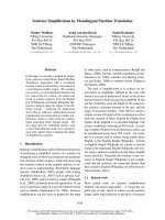
About 120 potential jurors were being asked to complete a lengthy questionnaire .
The jurors were taken into the courtroom in groups of 40 and asked to fill out a questionnaire .
Figure 2: Discovered alignment of Ex. 19 produced by G
p
. Observe that the model aligns identical words and also “complete”
and “fill” in this specific case. This kind of alignment provides an edge over a simple lexical overlap model.
“mostly bidirectional entailment,” a standard def-
inition of the paraphrase relation. Each sentence
was labeled first by two judges, who averaged 83%
agreement, and a third judge resolved conflicts.
We use the standard data split into 4,076 (2,753
paraphrase, 1,323 not) training and 1,725 (1147
paraphrase, 578 not) test pairs. We reserved a ran-
domly selected 1,075 training pairs for tuning.We
cite some examples from the training set here:
(18) Revenue in the first quarter of the year dropped 15
percent from the same period a year earlier.
With the scandal hanging over Stewart’s company,
revenue in the first quarter of the year dropped 15
percent from the same period a year earlier.
(19) About 120 potential jurors were being asked to
complete a lengthy questionnaire.
The jurors were taken into the courtroom in groups of

40 and asked to fill out a questionnaire.
Ex. 18 is a true paraphrase pair. Notice the high
lexical overlap between the two sentences (uni-
gram overlap of 100% in one direction and 72%
in the other). Ex. 19 is another true paraphrase
pair with much lower lexical overlap (unigram
overlap of 50% in one direction and 30% in the
other). Notice the use of similar-meaning phrases
and irrelevant modifiers that retain the same mean-
ing in both sentences, which a lexical overlap
model cannot capture easily, but a model like a QG
might. Also, in both pairs, the relationship cannot
be called total bidirectional equivalence because
there is some extra information in one sentence
which cannot be inferred from the other.
Ex. 20 was labeled “not paraphrase”:
(20) “There were a number of bureaucratic and
administrative missed signals - there’s not one person
who’s responsible here,” Gehman said.
In turning down the NIMA offer, Gehman said, “there
were a number of bureaucratic and administrative
missed signals here.
There is significant content overlap, making a de-
cision difficult for a na
¨
ıve lexical overlap classifier.
(In fact, p
Q
labels this example n while the lexical
overlap models label it p.)

The fact that negative examples in this corpus
were selected because of their high lexical over-
lap is important. It means that any discrimina-
tive model is expected to learn to distinguish mere
overlap from paraphrase. This seems appropriate,
but it does mean that the “not paraphrase” relation
ought to be denoted “not paraphrase but decep-
tively similar on the surface.” It is for this reason
that we use a special QG for the n relation.
5 Experimental Evaluation
Here we present our experimental evaluation using
p
Q
. We trained on the training set (3,001 pairs)
and tuned model metaparameters (C in Eq. 17)
and the effect of different feature sets on the de-
velopment set (1,075 pairs). We report accuracy
on the official MSRPC test dataset. If the poste-
rior probability p
Q
(p | s
1
, s
2
) is greater than 0.5,
the pair is labeled “paraphrase” (as in Eq. 1).
5.1 Baseline
We replicated a state-of-the-art baseline model for
comparison. Wan et al. (2006) report the best pub-
lished accuracy, to our knowledge, on this task,

using a support vector machine. Our baseline is
a reimplementation of Wan et al. (2006), using
features calculated directly from s
1
and s
2
with-
out recourse to any hidden structure: proportion
of word unigram matches, proportion of lemma-
tized unigram matches, BLEU score (Papineni et
al., 2001), BLEU score on lemmatized tokens, F
measure (Turian et al., 2003), difference of sen-
tence length, and proportion of dependency rela-
tion overlap. The SVM was trained to classify
positive and negative examples of paraphrase us-
ing SVM
light
(Joachims, 1999).
8
Metaparameters,
tuned on the development data, were the regu-
larization constant and the degree of the polyno-
mial kernel (chosen in [10
−5
, 10
2
] and 1–5 respec-
tively.).
9
It is unsurprising that the SVM performs very

well on the MSRPC because of the corpus creation
process (see Sec. 4) where an SVM was applied
as well, with very similar features and a skewed
decision process (Dolan and Brockett, 2005).
8

9
Our replication of the Wan et al. model is approxi-
mate, because we used different preprocessing tools: MX-
POST for POS tagging (Ratnaparkhi, 1996), MSTParser
for parsing (McDonald et al., 2005), and Dan Bikel’s
interface ( />˜
dbikel/
software.html#wn) to WordNet (Miller, 1995) for
lemmatization information. Tuning led to C = 17 and poly-
nomial degree 4.
473
Model Accuracy Precision Recall
baselines
all p 66.49 66.49 100.00
Wan et al. SVM (reported) 75.63 77.00 90.00
Wan et al. SVM (replication) 75.42 76.88 90.14
p
Q
lexical semantics features removed 68.64 68.84 96.51
all features 73.33 74.48 91.10
c-command disallowed (best; see text) 73.86 74.89 91.28
§6
p
L

75.36 78.12 87.44
product of experts 76.06 79.57 86.05
oracles
Wan et al. SVM and p
L
80.17 100.00 92.07
Wan et al. SVM and p
Q
83.42 100.00 96.60
p
Q
and p
L
83.19 100.00 95.29
Table 2: Accuracy,
p-class precision, and
p-class recall on the test
set (N = 1,725). See
text for differences in
implementation
between Wan et al. and
our replication; their
reported score does not
include the full test set.
5.2 Results
Tab. 2 shows performance achieved by the base-
line SVM and variations on p
Q
on the test set. We
performed a few feature ablation studies, evaluat-

ing on the development data. We removed the lex-
ical semantics component of the QG,
10
and disal-
lowed the syntactic configurations one by one, to
investigate which components of p
Q
contributes to
system performance. The lexical semantics com-
ponent is critical, as seen by the drop in accu-
racy from the table (without this component, p
Q
behaves almost like the “all p” baseline). We
found that the most important configurations are
“parent-child,” and “child-parent” while damage
from ablating other configurations is relatively
small. Most interestingly, disallowing the “c-
command” configuration resulted in the best ab-
solute accuracy, giving us the best version of p
Q
.
The c-command configuration allows more distant
nodes in a source sentence to align to parent-child
pairs in a target (see Fig. 1d). Allowing this con-
figuration guides the model in the wrong direction,
thus reducing test accuracy. We tried disallowing
more than one configuration at a time, without get-
ting improvements on development data. We also
tried ablating the WordNet relations, and observed
that the “identical-word” feature hurt the model

the most. Ablating the rest of the features did not
produce considerable changes in accuracy.
The development data-selected p
Q
achieves
higher recall by 1 point than Wan et al.’s SVM,
but has precision 2 points worse.
5.3 Discussion
It is quite promising that a linguistically-motivated
probabilistic model comes so close to a string-
similarity baseline, without incorporating string-
local phrases. We see several reasons to prefer
10
This is accomplished by eliminating lines 12 and 13 from
the definition of p
kid
and redefining p
word
to be the unigram
word distribution estimated from the Gigaword corpus, as in
G
0
, without the help of WordNet.
the more intricate QG to the straightforward SVM.
First, the QG discovers hidden alignments be-
tween words. Alignments have been leveraged in
related tasks such as textual entailment (Giampic-
colo et al., 2007); they make the model more inter-
pretable in analyzing system output (e.g., Fig. 2).
Second, the paraphrases of a sentence can be con-

sidered to be monolingual translations. We model
the paraphrase problem using a direct machine
translation model, thus providing a translation in-
terpretation of the problem. This framework could
be extended to permit paraphrase generation, or to
exploit other linguistic annotations, such as repre-
sentations of semantics (see, e.g., Qiu et al., 2006).
Nonetheless, the usefulness of surface overlap
features is difficult to ignore. We next provide an
efficient way to combine a surface model with p
Q
.
6 Product of Experts
Incorporating structural alignment and surface
overlap features inside a single model can make
exact inference infeasible. As an example, con-
sider features like n-gram overlap percentages that
provide cues of content overlap between two sen-
tences. One intuitive way of including these fea-
tures in a QG could be including these only at
the root of the target tree, i.e. while calculating
C(r, 0). These features have to be included in
estimating p
kid
, which has log-linear component
models (Eq. 7- 13). For these bigram or trigram
overlap features, a similar log-linear model has
to be normalized with a partition function, which
considers the (unnormalized) scores of all possible
target sentences, given the source sentence.

We therefore combine p
Q
with a lexical overlap
model that gives another posterior probability es-
timate p
L
(c | s
1
, s
2
) through a product of experts
(PoE; Hinton, 2002), p
J
(c | s
1
, s
2
)
=
p
Q
(c | s
1
, s
2
) × p
L
(c | s
1
, s

2
)

c

∈{p,n}
p
Q
(c

| s
1
, s
2
) × p
L
(c

| s
1
, s
2
)
(21)
474
Eq. 21 takes the product of the two models’ poste-
rior probabilities, then normalizes it to sum to one.
PoE models are used to efficiently combine several
expert models that individually constrain different
dimensions in high-dimensional data, the product

therefore constraining all of the dimensions. Com-
bining models in this way grants to each expert
component model the ability to “veto” a class by
giving it low probability; the most probable class
is the one that is least objectionable to all experts.
Probabilistic Lexical Overlap Model We de-
vised a logistic regression (LR) model incorpo-
rating 18 simple features, computed directly from
s
1
and s
2
, without modeling any hidden corre-
spondence. LR (like the QG) provides a proba-
bility distribution, but uses surface features (like
the SVM). The features are of the form precision
n
(number of n-gram matches divided by the num-
ber of n-grams in s
1
), recall
n
(number of n-gram
matches divided by the number of n-grams in s
2
)
and F
n
(harmonic mean of the previous two fea-
tures), where 1 ≤ n ≤ 3. We also used lemma-

tized versions of these features. This model gives
the posterior probability p
L
(c | s
1
, s
2
), where
c ∈ {p, n}. We estimated the model parameters
analogously to Eq. 17. Performance is reported in
Tab. 2; this model is on par with the SVM, though
trading recall in favor of precision. We view it as a
probabilistic simulation of the SVM more suitable
for combination with the QG.
Training the PoE Various ways of training a PoE
exist. We first trained p
Q
and p
L
separately as
described, then initialized the PoE with those pa-
rameters. We then continued training, maximizing
(unregularized) conditional likelihood.
Experiment We used p
Q
with the “c-command”
configuration excluded, and the LR model in the
product of experts. Tab. 2 includes the final re-
sults achieved by the PoE. The PoE model outper-
forms all the other models, achieving an accuracy

of 76.06%.
11
The PoE is conservative, labeling a
pair as p only if the LR and the QG give it strong
p probabilities. This leads to high precision, at the
expense of recall.
Oracle Ensembles Tab. 2 shows the results of
three different oracle ensemble systems that cor-
rectly classify a pair if either of the two individual
systems in the combination is correct. Note that
the combinations involving p
Q
achieve 83%, the
11
This accuracy is significant over p
Q
under a paired t-test
(p < 0.04), but is not significant over the SVM.
human agreement level for the MSRPC. The LR
and SVM are highly similar, and their oracle com-
bination does not perform as well.
7 Related Work
There is a growing body of research that uses the
MSRPC (Dolan et al., 2004; Quirk et al., 2004)
to build models of paraphrase. As noted, the most
successful work has used edit distance (Zhang and
Patrick, 2005) or bag-of-words features to mea-
sure sentence similarity, along with shallow syn-
tactic features (Finch et al., 2005; Wan et al., 2006;
Corley and Mihalcea, 2005). Qiu et al. (2006)

used predicate-argument annotations.
Most related to our approach, Wu (2005) used
inversion transduction grammars—a synchronous
context-free formalism (Wu, 1997)—for this task.
Wu reported only positive-class (p) precision (not
accuracy) on the test set. He obtained 76.1%,
while our PoE model achieves 79.6% on that mea-
sure. Wu’s model can be understood as a strict
hierarchical maximum-alignment method. In con-
trast, our alignments are soft (we sum over them),
and we do not require strictly isomorphic syntac-
tic structures. Most importantly, our approach is
founded on a stochastic generating process and es-
timated discriminatively for this task, while Wu
did not estimate any parameters from data at all.
8 Conclusion
In this paper, we have presented a probabilistic
model of paraphrase incorporating syntax, lexi-
cal semantics, and hidden loose alignments be-
tween two sentences’ trees. Though it fully de-
fines a generative process for both sentences and
their relationship, the model is discriminatively
trained to maximize conditional likelihood. We
have shown that this model is competitive for de-
termining whether there exists a semantic rela-
tionship between them, and can be improved by
principled combination with more standard lexical
overlap approaches.
Acknowledgments
The authors thank the three anonymous review-

ers for helpful comments and Alan Black, Freder-
ick Crabbe, Jason Eisner, Kevin Gimpel, Rebecca
Hwa, David Smith, and Mengqiu Wang for helpful
discussions. This work was supported by DARPA
grant NBCH-1080004.
475
References
Regina Barzilay and Lillian Lee. 2003. Learn-
ing to paraphrase: an unsupervised approach using
multiple-sequence alignment. In Proc. of NAACL.
Daniel M. Bikel, Richard L. Schwartz, and Ralph M.
Weischedel. 1999. An algorithm that learns what’s
in a name. Machine Learning, 34(1-3):211–231.
Chris Callison-Burch, Philipp Koehn, and Miles Os-
borne. 2006. Improved statistical machine transla-
tion using paraphrases. In Proc. of HLT-NAACL.
Courtney Corley and Rada Mihalcea. 2005. Mea-
suring the semantic similarity of texts. In Proc. of
ACL Workshop on Empirical Modeling of Semantic
Equivalence and Entailment.
William B. Dolan and Chris Brockett. 2005. Auto-
matically constructing a corpus of sentential para-
phrases. In Proc. of IWP.
Bill Dolan, Chris Quirk, and Chris Brockett. 2004.
Unsupervised construction of large paraphrase cor-
pora: exploiting massively parallel news sources. In
Proc. of COLING.
Andrew Finch, Young Sook Hwang, and Eiichiro
Sumita. 2005. Using machine translation evalua-
tion techniques to determine sentence-level seman-

tic equivalence. In Proc. of IWP.
Danilo Giampiccolo, Bernardo Magnini, Ido Dagan,
and Bill Dolan. 2007. The third PASCAL recog-
nizing textual entailment challenge. In Proc. of the
ACL-PASCAL Workshop on Textual Entailment and
Paraphrasing.
David Graff. 2003. English Gigaword. Linguistic
Data Consortium.
Geoffrey E. Hinton. 2002. Training products of ex-
perts by minimizing contrastive divergence. Neural
Computation, 14:1771–1800.
Thorsten Joachims. 1999. Making large-scale SVM
learning practical. In Advances in Kernel Methods -
Support Vector Learning. MIT Press.
Dong C. Liu and Jorge Nocedal. 1989. On the limited
memory BFGS method for large scale optimization.
Math. Programming (Ser. B), 45(3):503–528.
Erwin Marsi and Emiel Krahmer. 2005. Explorations
in sentence fusion. In Proc. of EWNLG.
Ryan McDonald, Koby Crammer, and Fernando
Pereira. 2005. Online large-margin training of de-
pendency parsers. In Proc. of ACL.
Kathleen R. McKeown. 1979. Paraphrasing using
given and new information in a question-answer sys-
tem. In Proc. of ACL.
I. Dan Melamed. 2004. Statistical machine translation
by parsing. In Proc. of ACL.
George A. Miller. 1995. Wordnet: a lexical database
for English. Commun. ACM, 38(11):39–41.
Kishore Papineni, Salim Roukos, Todd Ward, and Wei-

Jing Zhu. 2001. BLEU: a method for automatic
evaluation of machine translation. In Proc. of ACL.
Long Qiu, Min-Yen Kan, and Tat-Seng Chua. 2006.
Paraphrase recognition via dissimilarity significance
classification. In Proc. of EMNLP.
Chris Quirk, Chris Brockett, and William B. Dolan.
2004. Monolingual machine translation for para-
phrase generation. In Proc. of EMNLP.
Adwait Ratnaparkhi. 1996. A maximum entropy
model for part-of-speech tagging. In Proc. of
EMNLP.
David A. Smith and Jason Eisner. 2006. Quasi-
synchronous grammars: Alignment by soft projec-
tion of syntactic dependencies. In Proc. of the HLT-
NAACL Workshop on Statistical Machine Transla-
tion.
Joseph P. Turian, Luke Shen, and I. Dan Melamed.
2003. Evaluation of machine translation and its
evaluation. In Proc. of Machine Translation Summit
IX.
Stephen Wan, Mark Dras, Robert Dale, and C
´
ecile
Paris. 2006. Using dependency-based features to
take the “para-farce” out of paraphrase. In Proc. of
ALTW.
Mengqiu Wang, Noah A. Smith, and Teruko Mita-
mura. 2007. What is the Jeopardy model? a quasi-
synchronous grammar for QA. In Proc. of EMNLP-
CoNLL.

Dekai Wu. 1997. Stochastic inversion transduction
grammars and bilingual parsing of parallel corpora.
Comput. Linguist., 23(3).
Dekai Wu. 2005. Recognizing paraphrases and textual
entailment using inversion transduction grammars.
In Proc. of the ACL Workshop on Empirical Model-
ing of Semantic Equivalence and Entailment.
Hiroyasu Yamada and Yuji Matsumoto. 2003. Statis-
tical dependency analysis with support vector ma-
chines. In Proc. of IWPT.
Yitao Zhang and Jon Patrick. 2005. Paraphrase identi-
fication by text canonicalization. In Proc. of ALTW.
476