Báo cáo khoa học: "A global model for joint lemmatization and part-of-speech prediction" doc
Bạn đang xem bản rút gọn của tài liệu. Xem và tải ngay bản đầy đủ của tài liệu tại đây (645.06 KB, 9 trang )
Proceedings of the 47th Annual Meeting of the ACL and the 4th IJCNLP of the AFNLP, pages 486–494,
Suntec, Singapore, 2-7 August 2009.
c
2009 ACL and AFNLP
A global model for joint lemmatization and part-of-speech prediction
Kristina Toutanova
Microsoft Research
Redmond, WA 98052
Colin Cherry
Microsoft Research
Redmond, WA 98052
Abstract
We present a global joint model for
lemmatization and part-of-speech predic-
tion. Using only morphological lexicons
and unlabeled data, we learn a partially-
supervised part-of-speech tagger and a
lemmatizer which are combined using fea-
tures on a dynamically linked dependency
structure of words. We evaluate our
model on English, Bulgarian, Czech, and
Slovene, and demonstrate substantial im-
provements over both a direct transduction
approach to lemmatization and a pipelined
approach, which predicts part-of-speech
tags before lemmatization.
1 Introduction
The traditional problem of morphological analysis
is, given a word form, to predict the set of all of
its possible morphological analyses. A morpho-
logical analysis consists of a part-of-speech tag
(POS), possibly other morphological features, and
a lemma (basic form) corresponding to this tag and
features combination (see Table 1 for examples).
We address this problem in the setting where we
are given a morphological dictionary for training,
and can additionally make use of un-annotated text
in the language. We present a new machine learn-
ing model for this task setting.
In addition to the morphological analysis task
we are interested in performance on two subtasks:
tag-set prediction (predicting the set of possible
tags of words) and lemmatization (predicting the
set of possible lemmas). The result of these sub-
tasks is directly useful for some applications.
1
If
we are interested in the results of each of these two
1
Tag sets are useful, for example, as a basis of sparsity-
reducing features for text labeling tasks; lemmatization is
useful for information retrieval and machine translation from
a morphologically rich to a morphologically poor language,
where full analysis may not be important.
subtasks in isolation, we might build independent
solutions which ignore the other subtask.
In this paper, we show that there are strong de-
pendencies between the two subtasks and we can
improve performance on both by sharing infor-
mation between them. We present a joint model
for these two subtasks: it is joint not only in that
it performs both tasks simultaneously, sharing in-
formation, but also in that it reasons about multi-
ple words jointly. It uses component tag-set and
lemmatization models and combines their predic-
tions while incorporating joint features in a log-
linear model, defined on a dynamically linked de-
pendency structure of words.
The model is formalized in Section 5 and eval-
uated in Section 6. We report results on English,
Bulgarian, Slovene, and Czech and show that joint
modeling reduces the lemmatization error by up to
19%, the tag-prediction error by up to 26% and the
error on the complete morphological analysis task
by up to 22.6%.
2 Task formalization
The main task that we would like to solve is
as follows: given a lexicon L which contains
all morphological analyses for a set of words
{w
1
, . . . , w
n
}, learn to predict all morphological
analyses for other words which are outside of L.
In addition to the lexicon, we are allowed to make
use of unannotated text T in the language. We will
predict morphological analyses for words which
occur in T. Note that the task is defined on word
types and not on words in context.
A morphological analysis of a word w consists
of a (possibly structured) POS tag t, together with
one or several lemmas, which are the possible ba-
sic forms of w when it has tag t. As an exam-
ple, Table 1 illustrates the morphological analy-
ses of several words taken from the CELEX lexi-
cal database of English (Baayen et al., 1995) and
the Multext-East lexicon of Bulgarian (Erjavec,
2004). The Bulgarian words are transcribed in
486
Word Forms Morphological Analyses Tags Lemmas
tell verb base (VB), tell VB tell
told verb past tense (VBD), tell VBD,VBN tell
verb past participle (VBN), tell
tells verb present 3rd person sing (VBZ), tell VBZ tell
telling verb present continuous (VBG), tell VBG,JJ tell
adjective (JJ), telling telling
izpravena adjective fem sing indef (A–FS-N), izpraven A–FS-N izpraven
verb main part past sing fem pass indef (VMPS-SFP-N), izpravia VMPS-SFP-N izpravia
izpraviha verb main indicative 3rd person plural (VMIA3P), izpravia VMIA3P izpravia
Table 1: Examples of morphological analyses of words in English and Bulgarian.
Latin characters. Here by “POS tags” we mean
both simple main pos-tags such as noun or verb,
and detailed tags which include grammatical fea-
tures, such as VBZ for English indicating present
tense third person singular verb and A–FS-N for
Bulgarian indicating a feminine singular adjective
in indefinite form. In this work we predict only
main POS tags for the Multext-East languages, as
detailed tags were less useful for lemmatization.
Since the predicted elements are sets, we use
precision, recall, and F-measure (F1) to evaluate
performance. The two subtasks, tag-set prediction
and lemmatization are also evaluated in this way.
Table 1 shows the correct tag-sets and lemmas for
each of the example words in separate columns.
Our task setting differs from most work on lemma-
tization which uses either no or a complete rootlist
(Wicentowski, 2002; Dreyer et al., 2008).
2
We can
use all forms occurring in the unlabeled text T but
there are no guarantees about the coverage of the
target lemmas or the number of noise words which
may occur in T (see Table 2 for data statistics).
Our setting is thus more realistic since it is what
one would have in a real application scenario.
3 Related work
In work on morphological analysis using machine
learning, the task is rarely addressed in the form
described above. Some exceptions are the work
(Bosch and Daelemans, 1999) which presents a
model for segmenting, stemming, and tagging
words in Dutch, and requires the prediction of
all possible analyses, and (Antal van den Bosch
and Soudi, 2007) which similarly requires the pre-
diction of all morpho-syntactically annotated seg-
mentations of words for Arabic. As opposed to
2
These settings refer to the availability of a set of word
forms which are possible lemmas; in the no rootlist setting,
no other word forms in the language are given in addition to
the forms in the training set; in the complete rootlist setting,
a set of word forms which consists of exactly all correct lem-
mas for the words in the test set is given.
our work, these approaches do not make use of un-
labeled data and make predictions for each word
type in isolation.
In machine learning work on lemmatization for
highly inflective languages, it is most often as-
sumed that a word form and a POS tag are given,
and the task is to predict the set of corresponding
lemma(s) (Mooney and Califf, 1995; Clark, 2002;
Wicentowski, 2002; Erjavec and D
ˇ
zeroski, 2004;
Dreyer et al., 2008). In our task setting, we do
not assume the availability of gold-standard POS
tags. As a component model, we use a lemmatiz-
ing string transducer which is related to these ap-
proaches and draws on previous work in this and
related string transduction areas. Our transducer is
described in detail in Section 4.1.
Another related line of work approaches the dis-
ambiguation problem directly, where the task is
to predict the correct analysis of word-forms in
context (in sentences), and not all possible anal-
yses. In such work it is often assumed that the cor-
rect POS tags can be predicted with high accuracy
using labeled POS-disambiguated sentences (Er-
javec and D
ˇ
zeroski, 2004; Habash and Rambow,
2005). A notable exception is the work of (Adler
et al., 2008), which uses unlabeled data and a
morphological analyzer to learn a semi-supervised
HMM model for disambiguation in context, and
also guesses analyses for unknown words using a
guesser of likely POS-tags. It is most closely re-
lated to our work, but does not attempt to predict
all possible analyses, and does not have to tackle
a complex string transduction problem for lemma-
tization since segmentation is mostly sufficient for
the focus language of that study (Hebrew).
The idea of solving two related tasks jointly to
improve performance on both has been success-
ful for other pairs of tasks (e.g., (Andrew et al.,
2004)). Doing joint inference instead of taking a
pipeline approach has also been shown useful for
other problems (e.g., (Finkel et al., 2006; Cohen
and Smith, 2007)).
487
4 Component models
We use two component models as the basis of
addressing the task: one is a partially-supervised
POS tagger which is trained using L and the unla-
beled text T; the other is a lemmatizing transducer
which is trained from L and can use T. The trans-
ducer can optionally be given input POS tags in
training and testing, which can inform the lemma-
tization. The tagger is described in Section 4.2 and
the transducer is described in Section 4.1.
In a pipeline approach to combining the tagging
and lemmatization components, we first predict a
set of tags for each word using the tagger, and then
ask the lemmatizer to predict one lemma for each
of the possible tags. In a direct transduction ap-
proach to the lemmatization subtask, we train the
lemmatizer without access to tags and ask it to
predict a single lemma for each word in testing.
Our joint model, described in Section 5, is defined
in a re-ranking framework, and can choose from
among k-best predictions of tag-sets and lemmas
generated from the component tagger and lemma-
tizer models.
4.1 Morphological analyser
We employ a discriminative character transducer
as a component morphological analyzer. The input
to the transducer is an inflected word (the source)
and possibly an estimated part-of-speech; the out-
put is the lemma of the word (the target). The
transducer is similar to the one described by Ji-
ampojamarn et al. (2008) for letter-to-phoneme
conversion, but extended to allow for whole-word
features on both the input and the output. The core
of our engine is the dynamic programming algo-
rithm for monotone phrasal decoding (Zens and
Ney, 2004). The main feature of this algorithm is
its capability to transduce many consecutive char-
acters with a single operation; the same algorithm
is employed to tag subsequences in semi-Markov
CRFs (Sarawagi and Cohen, 2004).
We employ three main categories of features:
context, transition, and vocabulary (rootlist) fea-
tures. The first two are described in detail by Ji-
ampojamarn et al. (2008), while the final is novel
to this work. Context features are centered around
a transduction operation such as es → e, as em-
ployed in gives → give. Context features include
an indicator for the operation itself, conjoined with
indicators for all n-grams of source context within
a fixed window of the operation. We also employ a
copy feature that indicates if the operation simply
copies the source character, such as e → e. Tran-
sition features are our Markov, or n-gram features
on transduction operations. Vocabulary features
are defined on complete target words, according
to the frequency of said word in a provided unla-
beled text T. We have chosen to bin frequencies;
experiments on a development set suggested that
two indicators are sufficient: the first fires for any
word that occurred fewer than five times, while a
second also fires for those words that did not oc-
cur at all. By encoding our vocabulary in a trie and
adding the trie index to the target context tracked
by our dynamic programming chart, we can ef-
ficiently track these frequencies during transduc-
tion.
We incorporate the source part-of-speech tag by
appending it to each feature, thus the context fea-
ture es → e may become es → e, VBZ. To en-
able communication between the various parts-of-
speech, a universal set of unannotated features also
fires, regardless of the part-of-speech, acting as a
back-off model of how words in general behave
during stemming.
Linear weights are assigned to each of the trans-
ducer’s features using an averaged perceptron for
structure prediction (Collins, 2002). Note that
our features are defined in terms of the operations
employed during transduction, therefore to cre-
ate gold-standard feature vectors, we require not
only target outputs, but also derivations to pro-
duce those outputs. We employ a deterministic
heuristic to create these derivations; given a gold-
standard source-target pair, we construct a deriva-
tion that uses only trivial copy operations until
the first character mismatch. The remainder of
the transduction is performed with a single multi-
character replacement. For example, the deriva-
tion for living → live would be l → l, i → i,
v → v, ing → e. For languages with morpholo-
gies affecting more than just the suffix, one can
either develop a more complex heuristic, or deter-
mine the derivations using a separate aligner such
as that of Ristad and Yianilos (1998).
4.2 Tag-set prediction model
The tag-set model uses a training lexicon L and
unlabeled text T to learn to predict sets of tags
for words. It is based on the semi-supervised tag-
ging model of (Toutanova and Johnson, 2008). It
has two sub-models: one is an ambiguity class
488
or a tag-set model, which can assign probabili-
ties for possible sets of tags of words P
T SM
(ts|w)
and the other is a word context model, which can
assign probabilities P
CM
(contexts
w
|w, ts) to all
contexts of occurrence of word w in an unlabeled
text T. The word-context model is Bayesian and
utilizes a sparse Dirichlet prior on the distributions
of tags given words. In addition, it uses informa-
tion on a four word context of occurrences of w in
the unlabeled text.
Note that the (Toutanova and Johnson, 2008)
model is a tagger that assigns tags to occurrences
of words in the text, whereas we only need to pre-
dict sets of possible tags for word types, such as
the set {VBD, VBN} for the word told. Their com-
ponent sub-model P
T SM
predicts sets of tags and
it is possible to use it on its own, but by also us-
ing the context model we can take into account
information from the context of occurrence of
words and compute probabilities of tag-sets given
the observed occurrences in T. The two are com-
bined to make a prediction for a tag-set of a test
word w, given unlabeled text T, using Bayes rule:
p(ts|w) ∝ P
T SM
(ts|w)P
CM
(contexts
w
|w, ts).
We use a direct re-implementation of the word-
context model, using variational inference follow-
ing (Toutanova and Johnson, 2008). For the tag-
set sub-model, we employ a more sophisticated
approach. First, we learn a log-linear classifier in-
stead of a Naive Bayes model, and second, we use
features derived from related words appearing in
T. The possible classes predicted by the classifier
are as many as the observed tag-sets in L. The
sparsity is relieved by adding features for individ-
ual tags t which get shared across tag-sets contain-
ing t.
There are two types of features in the model:
(i) word-internal features: word suffixes, capital-
ization, existence of hyphen, and word prefixes
(such features were also used in (Toutanova and
Johnson, 2008)), and (ii) features based on re-
lated words. These latter features are inspired by
(Cucerzan and Yarowsky, 2000) and are defined as
follows: for a word w such as telling, there is an
indicator feature for every combination of two suf-
fixes α and β, such that there is a prefix p where
telling= pα and pβ exists in T. For example, if the
word tells is found in T, there would be a feature
for the suffixes α=ing,β=s that fires. The suffixes
are defined as all character suffixes up to length
three which occur with at least 100 words.
VBD VBN JJ VBD VBN
JJR NN
bounce
bouncer bounce
…
bounc
bouncer
boucer
f
bounce bounce
bounced bounced
VB NN VB
bounce bounce
… …
…
f
Figure 1: A small subset of the graphical model. The
tag-sets and lemmas active in the illustrated assignment are
shown in bold. The extent of joint features firing for the
lemma bounce is shown as a factor indicated by the blue cir-
cle and connected to the assignments of the three words.
5 A global joint model for morphological
analysis
The idea of this model is to jointly predict the set
of possible tags and lemmas of words. In addi-
tion to modeling dependencies between the tags
and lemmas of a single word, we incorporate de-
pendencies between the predictions for multiple
words. The dependencies among words are deter-
mined dynamically. Intuitively, if two words have
the same lemma, their tag-sets are dependent. For
example, imagine that we need to determine the
tag-set and lemmas of the word bouncer. The tag-
set model may guess that the word is an adjective
in comparative form, because of its suffix, and be-
cause its occurrences in T might not strongly in-
dicate that it is a noun. The lemmatizer can then
lemmatize the word like an adjective and come up
with bounce as a lemma. If the tag-set model is
fairly certain that bounce is not an adjective, but
is a verb or a noun, a joint model which looks si-
multaneously at the tags and lemmas of bouncer
and bounce will detect a problem with this assign-
ments and will be able to correct the tagging and
lemmatization error for bouncer.
The main source of information our joint model
uses is information about the assignments of all
words that have the same lemma l . If the tag-set
model is better able to predict the tags of some of
these words, the information can propagate to the
other words. If some of them are lemmatized cor-
rectly, the model can be pushed to lemmatize the
others correctly as well. Since the lemmas of test
words are not given, the dependencies between as-
489
signments of words are determined dynamically
by the currently chosen set of lemmas.
As an example, Figure 1 shows three sample
English words and their possible tag-sets and lem-
mas determined by the component models. It also
illustrates the dependencies between the variables
induced by the features of our model active for the
current (incorrect) assignment.
5.1 Formal model description
Given a set of test words w
1
, . . . w
n
and additional
word forms occurring in unlabeled data T, we de-
rive an extended set of words w
1
, . . . , w
m
which
contains the original test words and additional re-
lated words, which can provide useful information
about the test words. For example, if bouncer is a
test word and bounce and bounced occur in T these
two words can be added to the set of test words
because they can contribute to the classification
of bouncer. The algorithm for selecting related
words is simple: we add any word for which the
pipelined model predicts a lemma which is also
predicted as one of the top k lemmas for a word
from the test set.
We define a joint model over tag-sets and lem-
mas for all words in the extended set, using fea-
tures defined on a dynamically linked structure
of words and their assigned analyses. It is a re-
ranking model because the tag-sets and possible
lemmas are limited to the top k options provided
by the pipelined model.
3
Our model is defined
on a very large set of variables, each of which
can take a large set of values. For example, for
a test set of size about 4,000 words for Slovene an
additional about 9,000 words from T were added
to the extended set. Each of these words has a
corresponding variable which indicates its tag-set
and lemma assignment. The possible assignments
range over all combinations available from the tag-
ging and lemmatizer component models; using the
top three tag-sets per word and top three lemmas
per tag gives an average of around 11.2 possible
assignments per word. This is because the tag-
sets have about 1.2 tags on average and we need
to choose a lemma for each. While it is not the
case that all variables are connected to each other
by features, the connectivity structure can be com-
plex.
More formally, let ts
j
i
denote possible tag-sets
3
We used top three tag-sets and top three lemmas for each
tag for training.
for word w
i
, for j = 1 . . . k. Also, let l
i
(t)
j
de-
note the top lemmas for word w
i
given tag t. An
assignment of a tag-set and lemmas to a word w
i
consists of a choice of a tag-set, ts
i
(one of the
possible k tag-sets for the word) and, for each tag
t in the chosen tag-set, a choice of a lemma out
of the possible lemmas for that tag and word. For
brevity, we denote such joint assignment by tl
i
.
As a concrete example, in Figure 1, we can see the
current assignments for three words: the assigned
tag-sets are shown underlined and in bolded boxes
(e.g., for bounced, the tag-set {VBD,VBN} is cho-
sen; for both tags, the lemma bounce is assigned).
Other possible tag-sets and other possible lemmas
for each chosen tag are shown in greyed boxes.
Our joint model defines a distribution over as-
signments to all words w
1
, . . . , w
m
. The form of
the model is as follows:
P (tl
1
, . . . , tl
m
) =
e
F (tl
1
, ,tl
m
)
θ
tl
1
, ,tl
m
e
F (tl
1
, ,tl
m
)
θ
Here F denotes the vector of features defined
over an assignment for all words in the set and θ
is a vector of parameters for the features. Next we
detail the types of features used.
Word-local features. The aim of such features is
to look at the set of all tags assigned to a word to-
gether with all lemmas and capture coarse-grained
dependencies at this level. These features intro-
duce joint dependencies between the tags and lem-
mas of a word, but they are still local to the as-
signment of single words. One such feature is the
number of distinct lemmas assigned across the dif-
ferent tags in the assigned tag-set. Another such
feature is the above joined with the identity of
the tag-set. For example, if a word’s tag-set is
{VBD,VBN}, it will likely have the same lemma
for both tags and the number of distinct lemmas
will be one (e.g., the word bounced), whereas if it
has the tags VBG, JJ the lemmas will be distinct for
the two tags (e.g. telling). In this class of features
are also the log-probabilities from the tag-set and
lemmatizer models.
Non-local features. Our non-local features look,
for every lemma l, at all words which have that
lemma as the lemma for at least one of their as-
signed tags, and derive several predicates on the
joint assignment to these words. For example,
using our word graph in the figure, the lemma
bounce is assigned to bounced for tags VBD and
VBN, to bounce for tags VB and NN, and to
bouncer for tag JJR. One feature looks at the
combination of tags corresponding to the differ-
490
ent forms of the lemma. In this case this would
be [JJR,NN+VB-lem,VBD+VBN]. The feature also
indicates any word which is exactly equal to the
lemma with lem as shown for the NN and VB tags
corresponding to bounce. Our model learns a neg-
ative weight for this feature, because the lemma
of a word with tag JJR is most often a word with
at least one tag equal to JJ. A variant of this
feature also appends the final character of each
word, like this: [JJR+r,NN+VB+e-lem,VBD+VBN-
d]. This variant was helpful for the Slavic lan-
guages because when using only main POS tags,
the granularity of the feature is too coarse. An-
other feature simply counts the number of distinct
words having the same lemma, encouraging re-
using the same lemma for different words. An ad-
ditional feature fires for every distinct lemma, in
effect counting the number of assigned lemmas.
5.2 Training and inference
Since the model is defined to re-rank candidates
from other component models, we need two differ-
ent training sets: one for training the component
models, and another for training the joint model
features. This is because otherwise the accuracy
of the component models would be overestimated
by the joint model. Therefore, we train the com-
ponent models on the training lexicons LTrain and
select their hyperparameters on the LDev lexicons.
We then train the joint model on the LDev lexicons
and evaluate it on the LTest lexicons. When apply-
ing models to the LTest set, the component mod-
els are first retrained on the union of LTrain and
LDev so that all models can use the same amount
of training data, without giving unfair advantage
to the joint model. Such set-up is also used for
other re-ranking models (Collins, 2000).
For training the joint model, we maximize the
log-likelihood of the correct assignment to the
words in LDev, marginalizing over the assign-
ments of other related words added to the graph-
ical model. We compute the gradient approx-
imately by computing expectations of features
given the observed assignments and marginal ex-
pectations of features. For computing these ex-
pectations we use Gibbs sampling to sample com-
plete assignments to all words in the graph.
4
We
4
We start the Gibbs sampler by the assignments found by
the pipeline method and then use an annealing schedule to
find a neighborhood of high-likelihood assignments, before
taking about 10 complete samples from the graph to compute
expectations.
use gradient descent with a small learning rate, se-
lected to optimize the accuracy on the LDev set.
For finding a most likely assignment at test time,
we use the sampling procedure, this time using a
slower annealing schedule before taking a single
sample to output as a guessed answer.
For the Gibbs sampler, we need to sample an
assignment for each word in turn, given the current
assignments of all other words. Let us denote the
current assignment to all words except w
i
as tl
−i
.
The conditional probability of an assignment tl
i
for word w
i
is given by:
P (tl
i
|tl
−i
) =
e
F (tl
i
,tl
−i
)
θ
tl
i
e
F (tl
i
,tl
−i
)
θ
The summation in the denominator is over all
possible assignments for word w
i
. To compute
these quantities we need to consider only the fea-
tures involving the current word. Because of the
nature of the features in our model, it is possible
to isolate separate connected components which
do not share features for any assignment. If two
words do not share lemmas for any of their possi-
ble assignments, they will be in separate compo-
nents. Block sampling within a component could
be used if the component is relatively small; how-
ever, for the common case where there are five or
more words in a fully connected component ap-
proximate inference is necessary.
6 Experiments
6.1 Data
We use datasets for four languages: English, Bul-
garian, Slovene, and Czech. For each of the lan-
guages, we need a lexicon with morphological
analyses L and unlabeled text.
For English we derive the lexicon from CELEX
(Baayen et al., 1995), and for the other lan-
guages we use the Multext-East resources (Er-
javec, 2004). For English we use only open-class
words (nouns, verbs, adjectives, and adverbs), and
for the other languages we use words of all classes.
The unlabeled data for English we use is the union
of the Penn Treebank tagged WSJ data (Marcus et
al., 1993) and the BLLIP corpus.
5
For the rest of
the languages we use only the text of George Or-
well’s novel 1984, which is provided in morpho-
logically disambiguated form as part of Multext-
East (but we don’t use the annotations). Table 2
5
The BLLIP corpus contains approximately 30 million
words of automatically parsed WSJ data. We used these cor-
pora as plain text, without the annotations.
491
Lang LTrain LDev LTest Text
ws tl nf ws tl nf ws tl nf
Eng 5.2 1.5 0.3 7.4 1.4 0.8 7.4 1.4 0.8 320
Bgr 6.9 1.2 40.8 3.8 1.1 53.6 3.8 1.1 52.8 16.3
Slv 7.5 1.2 38.3 4.2 1.2 49.1 4.2 1.2 49.8 17.8
Cz 7.9 1.1 32.8 4.5 1.1 43.2 4.5 1.1 43.0 19.1
Table 2: Data sets used in experiments. The number of
word types (ws) is shown approximately in thousands. Also
shown are average number of complete analyses (tl) and per-
cent target lemmas not found in the unlabeled text (nf).
details statistics about the data set sizes for differ-
ent languages.
We use three different lexicons for each lan-
guage: one for training (LTrain), one for devel-
opment (LDev), and one for testing (LTest). The
global model weights are trained on the develop-
ment set as described in section 5.2. The lex-
icons are derived such that very frequent words
are likely to be in the training lexicon and less
frequent words in the dev and test lexicons, to
simulate a natural process of lexicon construction.
The English lexicons were constructed as follows:
starting with the full CELEX dictionary and the
text of the Penn Treebank corpus, take all word
forms appearing in the first 2000 sentences (and
are found in CELEX) to form the training lexi-
con, and then take all other words occurring in
the corpus and split them equally between the de-
velopment and test lexicons (every second word
is placed in the test set, in the order of first oc-
currence in the corpus). For the rest of the lan-
guages, the same procedure is applied, starting
with the full Multext-East lexicons and the text of
the novel 1984. Note that while it is not possi-
ble for training words to be included in the other
lexicons, it is possible for different forms of the
same lemma to be in different lexicons. The size
of the training lexicons is relatively small and we
believe this is a realistic scenario for application of
such models. In Table 2 we can see the number of
words in each lexicon and the unlabeled corpora
(by type), the average number of tag-lemma com-
binations per word,
6
as well as the percentage of
word lemmas which do not occur in the unlabeled
text. For English, the large majority of target lem-
mas are available in T (with only 0.8% missing),
whereas for the Multext-East languages around 40
to 50% of the target lemmas are not found in T;
this partly explains the lower performance on these
languages.
6
The tags are main tags for the Multext-East languages
and detailed tags for English.
Language Tag Model Tag Lem T+L
English none – 94.0 –
full 89.9 95.3 88.9
no unlab data 80.0 94.1 78.3
Bulgarian none – 73.2 –
full 87.9 79.9 75.3
no unlab data 80.2 76.3 70.4
Table 3: Development set results using different tag-set
models and pipelined prediction.
6.2 Evaluation of direct and pipelined models
for lemmatization
As a first experiment which motivates our joint
modeling approach, we present a comparison on
lemmatization performance in two settings: (i)
when no tags are used in training or testing by the
transducer, and (ii) when correct tags are used in
training and tags predicted by the tagging model
are used in testing. In this section, we report per-
formance on English and Bulgarian only. Compa-
rable performance on the other Multext-East lan-
guages is shown in Section 6.
Results are presented in Table 3. The experi-
ments are performed using LTrain for training and
LDev for testing. We evaluate the models on tag-
set F-measure (Tag), lemma-set F-measure(Lem)
and complete analysis F-measure (T+L). We show
the performance on lemmatization when tags are
not predicted (Tag Model is none), and when tags
are predicted by the tag-set model. We can see that
on both languages lemmatization is significantly
improved when a latent tag-set variable is used as
a basis for prediction: the relative error reduction
in Lem F-measure is 21.7% for English and 25%
for Bulgarian. For Bulgarian and the other Slavic
languages we predicted only main POS tags, be-
cause this resulted in better lemmatization perfor-
mance.
It is also interesting to evaluate the contribution
of the unlabeled data T to the performance of the
tag-set model. This can be achieved by remov-
ing the word-context sub-model of the tagger and
also removing related word features. The results
achieved in this setting for English and Bulgarian
are shown in the rows labeled “no unlab data”. We
can see that the tag-set F-measure of such models
is reduced by 8 to 9 points and the lemmatization
F-measure is similarly reduced. Thus a large por-
tion of the positive impact tagging has on lemma-
tization is due to the ability of tagging models to
exploit unlabeled data.
The results of this experiment show there are
strong dependencies between the tagging and
492
lemmatization subtasks, which a joint model could
exploit.
6.3 Evaluation of joint models
Since our joint model re-ranks candidates pro-
duced by the component tagger and lemmatizer,
there is an upper bound on the achievable perfor-
mance. We report these upper bounds for the four
languages in Table 4, at the rows which list m-best
oracle under Model. The oracle is computed using
five-best tag-set predictions and three-best lemma
predictions per tag. We can see that the oracle per-
formance on tag F-measure is quite high for all
languages, but the performance on lemmatization
and the complete task is close to only 90 percent
for the Slavic languages. As a second oracle we
also report the perfect tag oracle, which selects
the lemmas determined by the transducer using the
correct part-of-speech tags. This shows how well
we could do if we made the tagging model perfect
without changing the lemmatizer. For the Slavic
languages this is quite a bit lower than the m-best
oracles, showing that the majority of errors of the
pipelined approach cannot be fixed by simply im-
proving the tagging model. Our global model has
the potential to improve lemma assignments even
given correct tags, by sharing information among
multiple words.
The actual achieved performance for three dif-
ferent models is also shown. For comparison,
the lemmatization performance of the direct trans-
duction approach which makes no use of tags is
also shown. The pipelined models select one-
best tag-set predictions from the tagging model,
and the 1-best lemmas for each tag, like the mod-
els used in Section 6.2. The model name lo-
cal FS denotes a joint log-linear model which
has only word-internal features. Even with only
word-internal features, performance is improved
for most languages. The the highest improvement
is for Slovene and represents a 7.8% relative re-
duction in F-measure error on the complete task.
When features looking at the joint assignments
of multiple words are added, the model achieves
much larger improvements (models joint FS in the
Table) across all languages.
7
The highest overall
improvement compared to the pipelined approach
is again for Slovene and represents 22.6% reduc-
tion in error for the full task; the reduction is 40%
7
Since the optimization is stochastic, the results are av-
eraged over four runs. The standard deviations are between
0.02 and 0.11.
Language Model Tag Lem T+L
English tag oracle 100 98.9 98.7
English m-best oracle 97.9 99.0 97.5
English no tags – 94.3 –
English pipelined 90.9 95.9 90.0
English local FS 90.8 95.9 90.0
English joint FS 91.7 96.1 91.0
Bulgarian tag oracle 100 84.3 84.3
Bulgarian m-best oracle 98.4 90.7 89.9
Bulgarian no tags – 73.2 –
Bulgarian pipelined 87.9 78.5 74.6
Bulgarian local FS 88.9 79.2 75.8
Bulgarian joint FS 89.5 81.0 77.8
Slovene tag oracle 100 85.9 85.9
Slovene m-best oracle 98.7 91.2 90.5
Slovene no tags – 78.4 –
Slovene pipelined 89.7 82.1 78.3
Slovene local FS 90.8 82.7 80.0
Slovene joint FS 92.4 85.5 83.2
Czech tag oracle 100 83.2 83.2
Czech m-best oracle 98.1 88.7 87.4
Czech no tags – 78.7 –
Czech pipelined 92.3 80.7 77.5
Czech local FS 92.3 80.9 78.0
Czech joint FS 93.7 83.0 80.5
Table 4: Results on the test set achieved by joint and
pipelined models and oracles. The numbers represent tag-set
prediction F-measure (Tag), lemma-set prediction F-measure
(Lem) and F-measure on predicting complete tag, lemma
analysis sets (T+L).
relative to the upper bound achieved by the m-best
oracle. The smallest overall improvement is for
English, representing a 10% error reduction over-
all, which is still respectable. The larger improve-
ment for Slavic languages might be due to the fact
that there are many more forms of a single lemma
and joint reasoning allows us to pool information
across the forms.
7 Conclusion
In this paper we concentrated on the task of mor-
phological analysis, given a lexicon and unanno-
tated data. We showed that the tasks of tag pre-
diction and lemmatization are strongly dependent
and that by building state-of-the art models for
the two subtasks and performing joint inference
we can improve performance on both tasks. The
main contribution of our work was that we intro-
duced a joint model for the two subtasks which in-
corporates dependencies between predictions for
multiple word types. We described a set of fea-
tures and an approximate inference procedure for a
global log-linear model capturing such dependen-
cies, and demonstrated its effectiveness on English
and three Slavic languages.
Acknowledgements
We would like to thank Galen Andrew and Lucy Vander-
wende for useful discussion relating to this work.
493
References
Meni Adler, Yoav Goldberg, and Michael Elhadad. 2008.
Unsupervised lexicon-based resolution of unknown words
for full morpholological analysis. In Proceedings of ACL-
08: HLT.
Galen Andrew, Trond Grenager, and Christopher Manning.
2004. Verb sense and subcategorization: Using joint in-
ference to improve performance on complementary tasks.
In EMNLP.
Erwin Marsi Antal van den Bosch and Abdelhadi Soudi.
2007. Memory-based morphological analysis and part-
of-speech tagging of arabic. In Abdelhadi Soudi, An-
tal van den Bosch, and Gunter Neumann, editors, Arabic
Computational Morphology Knowledge-based and Em-
pirical Methods. Springer.
R. H. Baayen, R. Piepenbrock, and L. Gulikers. 1995. The
CELEX lexical database.
Antal Van Den Bosch and Walter Daelemans. 1999.
Memory-based morphological analysis. In Proceedings
of the 37th Annual Meeting of the Association for Compu-
tational Linguistics.
Alexander Clark. 2002. Memory-based learning of mor-
phology with stochastic transducers. In Proceedings of
the 40th Annual Meeting of the Association for Computa-
tional Linguistics (ACL), pages 513–520.
Shay B. Cohen and Noah A. Smith. 2007. Joint morpholog-
ical and syntactic disambiguation. In EMNLP.
Michael Collins. 2000. Discriminative reranking for natural
language parsing. In ICML.
M. Collins. 2002. Discriminative training methods for hid-
den markov models: Theory and experiments with percep-
tron algorithms. In EMNLP.
S. Cucerzan and D. Yarowsky. 2000. Language independent
minimally supervised induction of lexical probabilities. In
Proceedings of ACL 2000.
Markus Dreyer, Jason R. Smith, and Jason Eisner. 2008.
Latent-variable modeling of string transductions with
finite-state methods. In Proceedings of the Conference
on Empirical Methods in Natural Language Processing
(EMNLP), pages 1080–1089, Honolulu, October.
Toma
ˇ
z Erjavec and Sa
ˇ
ao D
ˇ
zeroski. 2004. Machine learn-
ing of morphosyntactic structure: lemmatizing unknown
Slovene words. Applied Artificial Intelligence, 18:17—
41.
Toma
ˇ
z Erjavec. 2004. Multext-east version 3: Multilingual
morphosyntactic specifications, lexicons and corpora. In
Proceedings of LREC-04.
Jenny Rose Finkel, Christopher D. Manning, and Andrew Y.
Ng. 2006. Solving the problem of cascading errors:
Approximate bayesian inference for linguistic annotation
pipelines. In EMNLP.
Nizar Habash and Owen Rambow. 2005. Arabic tokeniza-
tion, part-of-speech tagging and morphological disam-
biguation in one fell swoop. In Proceedings of the 43rd
Annual Meeting of the Association for Computational Lin-
guistics.
Sittichai Jiampojamarn, Colin Cherry, and Grzegorz Kon-
drak. 2008. Joint processing and discriminative training
for letter-to-phoneme conversion. In Proceedings of ACL-
08: HLT, pages 905–913, Columbus, Ohio, June.
M. Marcus, B. Santorini, and Marcinkiewicz. 1993. Build-
ing a large annotated coprus of english: the penn treebank.
Computational Linguistics, 19.
Raymond J. Mooney and Mary Elaine Califf. 1995. Induc-
tion of first-order decision lists: Results on learning the
past tense of english verbs. Journal of Artificial Intelli-
gence Research, 3:1—24.
Eric Sven Ristad and Peter N. Yianilos. 1998. Learning
string-edit distance. IEEE Transactions on Pattern Analy-
sis and Machine Intelligence, 20(5):522–532.
Sunita Sarawagi and William Cohen. 2004. Semimarkov
conditional random fields for information extraction. In
ICML.
Kristina Toutanova and Mark Johnson. 2008. A bayesian
LDA-based model for semi-supervised part-of-speech tag-
ging. In nips08.
Richard Wicentowski. 2002. Modeling and Learning Mul-
tilingual Inflectional Morphology in a Minimally Super-
vised Framework. Ph.D. thesis, Johns-Hopkins Univer-
sity.
R. Zens and H. Ney. 2004. Improvements in phrase-based
statistical machine translation. In HLT-NAACL, pages
257–264, Boston, USA, May.
494