Báo cáo khoa học: "An Error-Driven Word-Character Hybrid Model for Joint Chinese Word Segmentation and POS Tagging" docx
Bạn đang xem bản rút gọn của tài liệu. Xem và tải ngay bản đầy đủ của tài liệu tại đây (772.84 KB, 9 trang )
Proceedings of the 47th Annual Meeting of the ACL and the 4th IJCNLP of the AFNLP, pages 513–521,
Suntec, Singapore, 2-7 August 2009.
c
2009 ACL and AFNLP
An Error-Driven Word-Character Hybrid Model
for Joint Chinese Word Segmentation and POS Tagging
Canasai Kruengkrai
†‡
and Kiyotaka Uchimoto
‡
and Jun’ichi Kazama
‡
Yiou Wang
‡
and Kentaro Torisawa
‡
and Hitoshi Isahara
†‡
†
Graduate School of Engineering, Kobe University
1-1 Rokkodai-cho, Nada-ku, Kobe 657-8501 Japan
‡
National Institute of Information and Communications Technology
3-5 Hikaridai, Seika-cho, Soraku-gun, Kyoto 619-0289 Japan
{canasai,uchimoto,kazama,wangyiou,torisawa,isahara}@nict.go.jp
Abstract
In this paper, we present a discriminative
word-character hybrid model for joint Chi-
nese word segmentation and POS tagging.
Our word-character hybrid model offers
high performance since it can handle both
known and unknown words. We describe
our strategies that yield good balance for
learning the characteristics of known and
unknown words and propose an error-
driven policy that delivers such balance
by acquiring examples of unknown words
from particular errors in a training cor-
pus. We describe an efficient framework
for training our model based on the Mar-
gin Infused Relaxed Algorithm (MIRA),
evaluate our approach on the Penn Chinese
Treebank, and show that it achieves supe-
rior performance compared to the state-of-
the-art approaches reported in the litera-
ture.
1 Introduction
In Chinese, word segmentation and part-of-speech
(POS) tagging are indispensable steps for higher-
level NLP tasks. Word segmentation and POS tag-
ging results are required as inputs to other NLP
tasks, such as phrase chunking, dependency pars-
ing, and machine translation. Word segmenta-
tion and POS tagging in a joint process have re-
ceived much attention in recent research and have
shown improvements over a pipelined fashion (Ng
and Low, 2004; Nakagawa and Uchimoto, 2007;
Zhang and Clark, 2008; Jiang et al., 2008a; Jiang
et al., 2008b).
In joint word segmentation and the POS tag-
ging process, one serious problem is caused by
unknown words, which are defined as words that
are not found in a training corpus or in a sys-
tem’s word dictionary
1
. The word boundaries and
the POS tags of unknown words, which are very
difficult to identify, cause numerous errors. The
word-character hybrid model proposed by Naka-
gawa and Uchimoto (Nakagawa, 2004; Nakagawa
and Uchimoto, 2007) shows promising properties
for solving this problem. However, it suffers from
structural complexity. Nakagawa (2004) described
a training method based on a word-based Markov
model and a character-based maximum entropy
model that can be completed in a reasonable time.
However, this training method is limited by the
generatively-trained Markov model in which in-
formative features are hard to exploit.
In this paper, we overcome such limitations
concerning both efficiency and effectiveness. We
propose a new framework for training the word-
character hybrid model based on the Margin
Infused Relaxed Algorithm (MIRA) (Crammer,
2004; Crammer et al., 2005; McDonald, 2006).
We describe k-best decoding for our hybrid model
and design its loss function and the features appro-
priate for our task.
In our word-character hybrid model, allowing
the model to learn the characteristics of both
known and unknown words is crucial to achieve
optimal performance. Here, we describe our
strategies that yield good balance for learning
these two characteristics. We propose an error-
driven policy that delivers this balance by acquir-
ing examples of unknown words from particular
errors in a training corpus. We conducted our ex-
periments on Penn Chinese Treebank (Xia et al.,
2000) and compared our approach with the best
previous approaches reported in the literature. Ex-
perimental results indicate that our approach can
achieve state-of-the-art performance.
1
A system’s word dictionary usually consists of a word
list, and each word in the list has its own POS category. In
this paper, we constructed the system’s word dictionary from
a training corpus.
513
Figure 1: Lattice used in word-character hybrid model.
Tag Description
B Beginning character in a multi-character word
I Intermediate character in a multi-character word
E End character in a multi-character word
S Single-character word
Table 1: Position-of-character (POC) tags.
The paper proceeds as follows: Section 2 gives
background on the word-character hybrid model,
Section 3 describes our policies for correct path
selection, Section 4 presents our training method
based on MIRA, Section 5 shows our experimen-
tal results, Section 6 discusses related work, and
Section 7 concludes the paper.
2 Background
2.1 Problem formation
In joint word segmentation and the POS tag-
ging process, the task is to predict a path
of word hypotheses y = (y
1
, . . . , y
#y
) =
(w
1
, p
1
, . . . , w
#y
, p
#y
) for a given character
sequence x = (c
1
, . . . , c
#x
), where w is a word,
p is its POS tag, and a “#” symbol denotes the
number of elements in each variable. The goal of
our learning algorithm is to learn a mapping from
inputs (unsegmented sentences) x ∈ X to outputs
(segmented paths) y ∈ Y based on training sam-
ples of input-output pairs S = {(x
t
, y
t
)}
T
t=1
.
2.2 Search space representation
We represent the search space with a lattice based
on the word-character hybrid model (Nakagawa
and Uchimoto, 2007). In the hybrid model,
given an input sentence, a lattice that consists
of word-level and character-level nodes is con-
structed. Word-level nodes, which correspond to
words found in the system’s word dictionary, have
regular POS tags. Character-level nodes have spe-
cial tags where position-of-character (POC) and
POS tags are combined (Asahara, 2003; Naka-
gawa, 2004). POC tags indicate the word-internal
positions of the characters, as described in Table 1.
Figure 1 shows an example of a lattice for a Chi-
nese sentence: “ ” (Chongming is
China’s third largest island). Note that some nodes
and state transitions are not allowed. For example,
I and E nodes cannot occur at the beginning of the
lattice (marked with dashed boxes), and the transi-
tions from I to B nodes are also forbidden. These
nodes and transitions are ignored during the lattice
construction processing.
In the training phase, since several paths
(marked in bold) can correspond to the correct
analysis in the annotated corpus, we need to se-
lect one correct path y
t
as a reference for training.
2
The next section describes our strategies for deal-
ing with this issue.
With this search space representation, we
can consistently handle unknown words with
character-level nodes. In other words, we use
word-level nodes to identify known words and
character-level nodes to identify unknown words.
In the testing phase, we can use a dynamic pro-
gramming algorithm to search for the most likely
path out of all candidate paths.
2
A machine learning problem exists called structured
multi-label classification that allows training from multiple
correct paths. However, in this paper we limit our considera-
tion to structured single-label classification, which is simple
yet provides great performance.
514
3 Policies for correct path selection
In this section, we describe our strategies for se-
lecting the correct path y
t
in the training phase.
As shown in Figure 1, the paths marked in bold
can represent the correct annotation of the seg-
mented sentence. Ideally, we need to build a word-
character hybrid model that effectively learns the
characteristics of unknown words (with character-
level nodes) as well as those of known words (with
word-level nodes).
We can directly estimate the statistics of known
words from an annotated corpus where a sentence
is already segmented into words and assigned POS
tags. If we select the correct path y
t
that corre-
sponds to the annotated sentence, it will only con-
sist of word-level nodes that do not allow learning
for unknown words. We therefore need to choose
character-level nodes as correct nodes instead of
word-level nodes for some words. We expect that
those words could reflect unknown words in the
future.
Baayen and Sproat (1996) proposed that the
characteristics of infrequent words in a training
corpus resemble those of unknown words. Their
idea has proven effective for estimating the statis-
tics of unknown words in previous studies (Ratna-
parkhi, 1996; Nagata, 1999; Nakagawa, 2004).
We adopt Baayen and Sproat’s approach as
the baseline policy in our word-character hybrid
model. In the baseline policy, we first count the
frequencies of words
3
in the training corpus. We
then collect infrequent words that appear less than
or equal to r times.
4
If these infrequent words are
in the correct path, we use character-level nodes
to represent them, and hence the characteristics of
unknown words can be learned. For example, in
Figure 1 we select the character-level nodes of the
word “ ” (Chongming) as the correct nodes. As
a result, the correct path y
t
can contain both word-
level and character-level nodes (marked with as-
terisks (*)).
To discover more statistics of unknown words,
one might consider just increasing the threshold
value r to obtain more artificial unknown words.
However, our experimental results indicate that
our word-character hybrid model requires an ap-
propriate balance between known and artificial un-
3
We consider a word and its POS tag a single entry.
4
In our experiments, the optimal threshold value r is se-
lected by evaluating the performance of joint word segmen-
tation and POS tagging on the development set.
known words to achieve optimal performance.
We now describe our new approach to lever-
age additional examples of unknown words. In-
tuition suggests that even though the system can
handle some unknown words, many unidentified
unknown words remain that cannot be recovered
by the system; we wish to learn the characteristics
of such unidentified unknown words. We propose
the following simple scheme:
• Divide the training corpus into ten equal sets
and perform 10-fold cross validation to find
the errors.
• For each trial, train the word-character hybrid
model with the baseline policy (r = 1) us-
ing nine sets and estimate errors using the re-
maining validation set.
• Collect unidentified unknown words from
each validation set.
Several types of errors are produced by the
baseline model, but we only focus on those caused
by unidentified unknown words, which can be eas-
ily collected in the evaluation process. As de-
scribed later in Section 5.2, we measure the recall
on out-of-vocabulary (OOV) words. Here, we de-
fine unidentified unknown words as OOV words
in each validation set that cannot be recovered by
the system. After ten cross validation runs, we
get a list of the unidentified unknown words de-
rived from the whole training corpus. Note that
the unidentified unknown words in the cross val-
idation are not necessary to be infrequent words,
but some overlap may exist. Finally, we obtain the
artificial unknown words that combine the uniden-
tified unknown words in cross validation and in-
frequent words for learning unknown words. We
refer to this approach as the error-driven policy.
4 Training method
4.1 Discriminative online learning
Let Y
t
= {y
1
t
, . . . , y
K
t
} be a lattice consisting of
candidate paths for a given sentence x
t
. In the
word-character hybrid model, the lattice Y
t
can
contain more than 1000 nodes, depending on the
length of the sentence x
t
and the number of POS
tags in the corpus. Therefore, we require a learn-
ing algorithm that can efficiently handle large and
complex lattice structures.
Online learning is an attractive method for
the hybrid model since it quickly converges
515
Algorithm 1 Generic Online Learning Algorithm
Input: Training set S = {(x
t
, y
t
)}
T
t=1
Output: Model weight vector w
1: w
(0)
= 0; v = 0; i = 0
2: for iter = 1 to N do
3: for t = 1 to T do
4: w
(i+1)
= update w
(i)
according to (x
t
, y
t
)
5: v = v + w
(i+1)
6: i = i + 1
7: end for
8: end for
9: w = v/(N ×T )
within a few iterations (McDonald, 2006). Algo-
rithm 1 outlines the generic online learning algo-
rithm (McDonald, 2006) used in our framework.
4.2 k-best MIRA
We focus on an online learning algorithm called
MIRA (Crammer, 2004), which has the de-
sired accuracy and scalability properties. MIRA
combines the advantages of margin-based and
perceptron-style learning with an optimization
scheme. In particular, we use a generalized ver-
sion of MIRA (Crammer et al., 2005; McDonald,
2006) that can incorporate k-best decoding in the
update procedure. To understand the concept of k-
best MIRA, we begin with a linear score function:
s(x, y; w) = w, f(x, y) , (1)
where w is a weight vector and f is a feature rep-
resentation of an input x and an output y.
Learning a mapping between an input-output
pair corresponds to finding a weight vector w such
that the best scoring path of a given sentence is
the same as (or close to) the correct path. Given
a training example (x
t
, y
t
), MIRA tries to estab-
lish a margin between the score of the correct path
s(x
t
, y
t
; w ) and the score of the best candidate
path s(x
t
,
ˆ
y; w) based on the current weight vector
w that is proportional to a loss function L(y
t
,
ˆ
y).
In each iteration, MIRA updates the weight vec-
tor w by keeping the norm of the change in the
weight vector as small as possible. With this
framework, we can formulate the optimization
problem as follows (McDonald, 2006):
w
(i+1)
= argmin
w
w − w
(i)
(2)
s.t. ∀
ˆ
y ∈ best
k
(x
t
; w
(i)
) :
s(x
t
, y
t
; w ) − s(x
t
,
ˆ
y; w) ≥ L(y
t
,
ˆ
y) ,
where best
k
(x
t
; w
(i)
) ∈ Y
t
represents a set of top
k-best paths given the weight vector w
(i)
. The
above quadratic programming (QP) problem can
be solved using Hildreth’s algorithm (Yair Cen-
sor, 1997). Replacing Eq. (2) into line 4 of Al-
gorithm 1, we obtain k-best MIRA.
The next question is how to efficiently gener-
ate best
k
(x
t
; w
(i)
). In this paper, we apply a dy-
namic programming search (Nagata, 1994) to k-
best MIRA. The algorithm has two main search
steps: forward and backward. For the forward
search, we use Viterbi-style decoding to find the
best partial path and its score up to each node in
the lattice. For the backward search, we use A
∗
-
style decoding to generate the top k-best paths. A
complete path is found when the backward search
reaches the beginning node of the lattice, and the
algorithm terminates when the number of gener-
ated paths equals k.
In summary, we use k-best MIRA to iteratively
update w
(i)
. The final weight vector w is the av-
erage of the weight vectors after each iteration.
As reported in (Collins, 2002; McDonald et al.,
2005), parameter averaging can effectively avoid
overfitting. For inference, we can use Viterbi-style
decoding to search for the most likely path y
∗
for
a given sentence x where:
y
∗
= argmax
y∈Y
s(x, y; w) . (3)
4.3 Loss function
In conventional sequence labeling where the ob-
servation sequence (word) boundaries are fixed,
one can use the 0/1 loss to measure the errors of
a predicted path with respect to the correct path.
However, in our model, word boundaries vary
based on the considered path, resulting in a dif-
ferent numbers of output tokens. As a result, we
cannot directly use the 0/1 loss.
We instead compute the loss function through
false positives (F P) and false negatives (F N).
Here, FP means the number of output nodes that
are not in the correct path, and FN means the
number of nodes in the correct path that cannot
be recognized by the system. We define the loss
function by:
L(y
t
,
ˆ
y) = F P + F N . (4)
This loss function can reflect how bad the pre-
dicted path
ˆ
y is compared to the correct path y
t
.
A weighted loss function based on F P and F N
can be found in (Ganchev et al., 2007).
516
ID Template Condition
W0 w
0
for word-level
W1 p
0
nodes
W2 w
0
, p
0
W3 Length(w
0
), p
0
A0 A
S
(w
0
) if w
0
is a single-
A1 A
S
(w
0
), p
0
character word
A2 A
B
(w
0
) for word-level
A3 A
B
(w
0
), p
0
nodes
A4 A
E
(w
0
)
A5 A
E
(w
0
), p
0
A6 A
B
(w
0
), A
E
(w
0
)
A7 A
B
(w
0
), A
E
(w
0
), p
0
T0 T
S
(w
0
) if w
0
is a single-
T1 T
S
(w
0
), p
0
character word
T2 T
B
(w
0
) for word-level
T3 T
B
(w
0
), p
0
nodes
T4 T
E
(w
0
)
T5 T
E
(w
0
), p
0
T6 T
B
(w
0
), T
E
(w
0
)
T7 T
B
(w
0
), T
E
(w
0
), p
0
C0 c
j
, j ∈ [−2, 2] × p
0
for character-
C1 c
j
, c
j+1
, j ∈ [−2, 1] × p
0
level nodes
C2 c
−1
, c
1
× p
0
C3 T (c
j
), j ∈ [−2, 2] × p
0
C4 T (c
j
), T(c
j+1
), j ∈ [−2, 1] × p
0
C5 T (c
−1
), T(c
1
) × p
0
C6 c
0
, T(c
0
) × p
0
Table 2: Unigram features.
4.4 Features
This section discusses the structure of f(x, y). We
broadly classify features into two categories: uni-
gram and bigram features. We design our feature
templates to capture various levels of information
about words and POS tags. Let us introduce some
notation. We write w
−1
and w
0
for the surface
forms of words, where subscripts −1 and 0 in-
dicate the previous and current positions, respec-
tively. POS tags p
−1
and p
0
can be interpreted in
the same way. We denote the characters by c
j
.
Unigram features: Table 2 shows our unigram
features. Templates W0–W3 are basic word-level
unigram features, where Length(w
0
) denotes the
length of the word w
0
. Using just the surface
forms can overfit the training data and lead to poor
predictions on the test data. To alleviate this prob-
lem, we use two generalized features of the sur-
face forms. The first is the beginning and end
characters of the surface (A0–A7). For example,
A
B
(w
0
) denotes the beginning character of the
current word w
0
, and A
B
(w
0
), A
E
(w
0
) denotes
the beginning and end characters in the word. The
second is the types of beginning and end charac-
ters of the surface (T0–T7). We define a set of
general character types, as shown in Table 4.
Templates C0–C6 are basic character-level un-
ID Template Condition
B0 w
−1
, w
0
if w
−1
and w
0
B1 p
−1
, p
0
are word-level
B2 w
−1
, p
0
nodes
B3 p
−1
, w
0
B4 w
−1
, w
0
, p
0
B5 p
−1
, w
0
, p
0
B6 w
−1
, p
−1
, w
0
B7 w
−1
, p
−1
, p
0
B8 w
−1
, p
−1
, w
0
, p
0
B9 Length(w
−1
), p
0
TB0 T
E
(w
−1
)
TB1 T
E
(w
−1
), p
0
TB2 T
E
(w
−1
), p
−1
, p
0
TB3 T
E
(w
−1
), T
B
(w
0
)
TB4 T
E
(w
−1
), T
B
(w
0
), p
0
TB5 T
E
(w
−1
), p
−1
, T
B
(w
0
)
TB6 T
E
(w
−1
), p
−1
, T
B
(w
0
), p
0
CB0 p
−1
, p
0
otherwise
Table 3: Bigram features.
Character type Description
Space Space
Numeral Arabic and Chinese numerals
Symbol Symbols
Alphabet Alphabets
Chinese Chinese characters
Other Others
Table 4: Character types.
igram features taken from (Nakagawa, 2004).
These templates operate over a window of ±2
characters. The features include characters (C0),
pairs of characters (C1–C2), character types (C3),
and pairs of character types (C4–C5). In addi-
tion, we add pairs of characters and character types
(C6).
Bigram features: Table 3 shows our bigram
features. Templates B0-B9 are basic word-
level bigram features. These features aim to
capture all the possible combinations of word
and POS bigrams. Templates TB0-TB6 are the
types of characters for bigrams. For example,
T
E
(w
−1
), T
B
(w
0
) captures the change of char-
acter types from the end character in the previ-
ous word to the beginning character in the current
word.
Note that if one of the adjacent nodes is a
character-level node, we use the template CB0 that
represents POS bigrams. In our preliminary ex-
periments, we found that if we add more features
to non-word-level bigrams, the number of features
grows rapidly due to the dense connections be-
tween non-word-level nodes. However, these fea-
tures only slightly improve performance over us-
ing simple POS bigrams.
517
(a) Experiments on small training corpus
Data set CTB chap. IDs # of sent. # of words
Training 1-270 3,046 75,169
Development 301-325 350 6,821
Test 271-300 348 8,008
# of POS tags 32
OOV (word) 0.0987 (790/8,008)
OOV (word & POS) 0.1140 (913/8,008)
(b) Experiments on large training corpus
Data set CTB chap. IDs # of sent. # of words
Training 1-270, 18,089 493,939
400-931,
1001-1151
Development 301-325 350 6,821
Test 271-300 348 8,008
# of POS tags 35
OOV (word) 0.0347 (278/8,008)
OOV (word & POS) 0.0420 (336/8,008)
Table 5: Training, development, and test data
statistics on CTB 5.0 used in our experiments.
5 Experiments
5.1 Data sets
Previous studies on joint Chinese word segmen-
tation and POS tagging have used Penn Chinese
Treebank (CTB) (Xia et al., 2000) in experiments.
However, versions of CTB and experimental set-
tings vary across different studies.
In this paper, we used CTB 5.0 (LDC2005T01)
as our main corpus, defined the training, develop-
ment and test sets according to (Jiang et al., 2008a;
Jiang et al., 2008b), and designed our experiments
to explore the impact of the training corpus size on
our approach. Table 5 provides the statistics of our
experimental settings on the small and large train-
ing data. The out-of-vocabulary (OOV) is defined
as tokens in the test set that are not in the train-
ing set (Sproat and Emerson, 2003). Note that the
development set was only used for evaluating the
trained model to obtain the optimal values of tun-
able parameters.
5.2 Evaluation
We evaluated both word segmentation (Seg) and
joint word segmentation and POS tagging (Seg
& Tag). We used recall (R), precision (P ), and
F
1
as evaluation metrics. Following (Sproat and
Emerson, 2003), we also measured the recall on
OOV (R
OOV
) tokens and in-vocabulary (R
IV
) to-
kens. These performance measures can be calcu-
lated as follows:
Recall (R) =
# of correct tokens
# of tokens in test data
P recision (P ) =
# of correct tokens
# of tokens in system output
F
1
=
2 · R · P
R + P
R
OOV
=
# of correct OOV tokens
# of OOV tokens in test data
R
IV
=
# of correct IV tokens
# of IV tokens in test data
For Seg, a token is considered to be a cor-
rect one if the word boundary is correctly iden-
tified. For Seg & Tag, both the word boundary and
its POS tag have to be correctly identified to be
counted as a correct token.
5.3 Parameter estimation
Our model has three tunable parameters: the num-
ber of training iterations N; the number of top
k-best paths; and the threshold r for infrequent
words. Since we were interested in finding an
optimal combination of word-level and character-
level nodes for training, we focused on tuning r.
We fixed N = 10 and k = 5 for all experiments.
For the baseline policy, we varied r in the range
of [1, 5] and found that setting r = 3 yielded the
best performance on the development set for both
the small and large training corpus experiments.
For the error-driven policy, we collected unidenti-
fied unknown words using 10-fold cross validation
on the training set, as previously described in Sec-
tion 3.
5.4 Impact of policies for correct path
selection
Table 6 shows the results of our word-character
hybrid model using the error-driven and baseline
policies. The third and fourth columns indicate the
numbers of known and artificial unknown words
in the training phase. The total number of words
is the same, but the different policies yield differ-
ent balances between the known and artificial un-
known words for learning the hybrid model. Op-
timal balances were selected using the develop-
ment set. The error-driven policy provides addi-
tional artificial unknown words in the training set.
The error-driven policy can improve R
OOV
as well
as maintain good R
IV
, resulting in overall F
1
im-
provements.
518
(a) Experiments on small training corpus
# of words in training (75,169)
Eval type Policy kwn. art. unk. R P F
1
R
OOV
R
IV
Seg
error-driven 63,997 11,172 0.9587 0.9509 0.9548 0.7557 0.9809
baseline 64,999 10,170 0.9572 0.9489 0.9530 0.7304 0.9820
Seg & Tag
error-driven 63,997 11,172 0.8929 0.8857 0.8892 0.5444 0.9377
baseline 64,999 10,170 0.8897 0.8820 0.8859 0.5246 0.9367
(b) Experiments on large training corpus
# of words in training (493,939)
Eval Type Policy kwn. art. unk. R P F
1
R
OOV
R
IV
Seg
error-driven 442,423 51,516 0.9829 0.9746 0.9787 0.7698 0.9906
baseline 449,679 44,260 0.9821 0.9736 0.9779 0.7590 0.9902
Seg & Tag
error-driven 442,423 51,516 0.9407 0.9328 0.9367 0.5982 0.9557
baseline 449,679 44,260 0.9401 0.9319 0.9360 0.5952 0.9552
Table 6: Results of our word-character hybrid model using error-driven and baseline policies.
Method Seg Seg & Tag
Ours (error-driven) 0.9787 0.9367
Ours (baseline) 0.9779 0.9360
Jiang08a 0.9785 0.9341
Jiang08b 0.9774 0.9337
N&U07 0.9783 0.9332
Table 7: Comparison of F
1
results with previous
studies on CTB 5.0.
Seg Seg & Tag
N&U07 Z&C08 Ours N&U07 Z&C08 Ours
Trial (base.) (base.)
1 0.9701 0.9721 0.9732 0.9262 0.9346 0.9358
2 0.9738 0.9762 0.9752 0.9318 0.9385 0.9380
3 0.9571 0.9594 0.9578 0.9023 0.9086 0.9067
4 0.9629 0.9592 0.9655 0.9132 0.9160 0.9223
5 0.9597 0.9606 0.9617 0.9132 0.9172 0.9187
6 0.9473 0.9456 0.9460 0.8823 0.8883 0.8885
7 0.9528 0.9500 0.9562 0.9003 0.9051 0.9076
8 0.9519 0.9512 0.9528 0.9002 0.9030 0.9062
9 0.9566 0.9479 0.9575 0.8996 0.9033 0.9052
10 0.9631 0.9645 0.9659 0.9154 0.9196 0.9225
Avg. 0.9595 0.9590 0.9611 0.9085 0.9134 0.9152
Table 8: Comparison of F
1
results of our baseline
model with Nakagawa and Uchimoto (2007) and
Zhang and Clark (2008) on CTB 3.0.
Method Seg Seg & Tag
Ours (baseline) 0.9611 0.9152
Z&C08 0.9590 0.9134
N&U07 0.9595 0.9085
N&L04 0.9520 -
Table 9: Comparison of averaged F
1
results (by
10-fold cross validation) with previous studies on
CTB 3.0.
5.5 Comparison with best prior approaches
In this section, we attempt to make meaning-
ful comparison with the best prior approaches re-
ported in the literature. Although most previous
studies used CTB, their versions of CTB and ex-
perimental settings are different, which compli-
cates comparison.
Ng and Low (2004) (N&L04) used CTB 3.0.
However, they just showed POS tagging results
on a per character basis, not on a per word basis.
Zhang and Clark (2008) (Z&C08) generated CTB
3.0 from CTB 4.0. Jiang et al. (2008a; 2008b)
(Jiang08a, Jiang08b) used CTB 5.0. Shi and
Wang (2007) used CTB that was distributed in the
SIGHAN Bakeoff. Besides CTB, they also used
HowNet (Dong and Dong, 2006) to obtain seman-
tic class features. Zhang and Clark (2008) indi-
cated that their results cannot directly compare to
the results of Shi and Wang (2007) due to different
experimental settings.
We decided to follow the experimental settings
of Jiang et al. (2008a; 2008b) on CTB 5.0 and
Zhang and Clark (2008) on CTB 4.0 since they
reported the best performances on joint word seg-
mentation and POS tagging using the training ma-
terials only derived from the corpora. The perfor-
mance scores of previous studies are directly taken
from their papers. We also conducted experiments
using the system implemented by Nakagawa and
Uchimoto (2007) (N&U07) for comparison.
Our experiment on the large training corpus is
identical to that of Jiang et al. (Jiang et al., 2008a;
Jiang et al., 2008b). Table 7 compares the F
1
re-
sults with previous studies on CTB 5.0. The result
of our error-driven model is superior to previous
reported results for both Seg and Seg & Tag, and
the result of our baseline model compares favor-
ably to the others.
Following Zhang and Clark (2008), we first
generated CTB 3.0 from CTB 4.0 using sentence
IDs 1–10364. We then divided CTB 3.0 into
ten equal sets and conducted 10-fold cross vali-
519
dation. Unfortunately, Zhang and Clark’s exper-
imental setting did not allow us to use our error-
driven policy since performing 10-fold cross val-
idation again on each main cross validation trial
is computationally too expensive. Therefore, we
used our baseline policy in this setting and fixed
r = 3 for all cross validation runs. Table 8 com-
pares the F
1
results of our baseline model with
Nakagawa and Uchimoto (2007) and Zhang and
Clark (2008) on CTB 3.0. Table 9 shows a sum-
mary of averaged F
1
results on CTB 3.0. Our
baseline model outperforms all prior approaches
for both Seg and Seg & Tag, and we hope that
our error-driven model can further improve perfor-
mance.
6 Related work
In this section, we discuss related approaches
based on several aspects of learning algorithms
and search space representation methods. Max-
imum entropy models are widely used for word
segmentation and POS tagging tasks (Uchimoto
et al., 2001; Ng and Low, 2004; Nakagawa,
2004; Nakagawa and Uchimoto, 2007) since they
only need moderate training times while they pro-
vide reasonable performance. Conditional random
fields (CRFs) (Lafferty et al., 2001) further im-
prove the performance (Kudo et al., 2004; Shi
and Wang, 2007) by performing whole-sequence
normalization to avoid label-bias and length-bias
problems. However, CRF-based algorithms typ-
ically require longer training times, and we ob-
served an infeasible convergence time for our hy-
brid model.
Online learning has recently gained popularity
for many NLP tasks since it performs comparably
or better than batch learning using shorter train-
ing times (McDonald, 2006). For example, a per-
ceptron algorithm is used for joint Chinese word
segmentation and POS tagging (Zhang and Clark,
2008; Jiang et al., 2008a; Jiang et al., 2008b).
Another potential algorithm is MIRA, which in-
tegrates the notion of the large-margin classifier
(Crammer, 2004). In this paper, we first intro-
duce MIRA to joint word segmentation and POS
tagging and show very encouraging results. With
regard to error-driven learning, Brill (1995) pro-
posed a transformation-based approach that ac-
quires a set of error-correcting rules by comparing
the outputs of an initial tagger with the correct an-
notations on a training corpus. Our approach does
not learn the error-correcting rules. We only aim to
capture the characteristics of unknown words and
augment their representatives.
As for search space representation, Ng and
Low (2004) found that for Chinese, the character-
based model yields better results than the word-
based model. Nakagawa and Uchimoto (2007)
provided empirical evidence that the character-
based model is not always better than the word-
based model. They proposed a hybrid approach
that exploits both the word-based and character-
based models. Our approach overcomes the limi-
tation of the original hybrid model by a discrimi-
native online learning algorithm for training.
7 Conclusion
In this paper, we presented a discriminative word-
character hybrid model for joint Chinese word
segmentation and POS tagging. Our approach
has two important advantages. The first is ro-
bust search space representation based on a hy-
brid model in which word-level and character-
level nodes are used to identify known and un-
known words, respectively. We introduced a sim-
ple scheme based on the error-driven concept to
effectively learn the characteristics of known and
unknown words from the training corpus. The sec-
ond is a discriminative online learning algorithm
based on MIRA that enables us to incorporate ar-
bitrary features to our hybrid model. Based on ex-
tensive comparisons, we showed that our approach
is superior to the existing approaches reported in
the literature. In future work, we plan to apply
our framework to other Asian languages, includ-
ing Thai and Japanese.
Acknowledgments
We would like to thank Tetsuji Nakagawa for his
helpful suggestions about the word-character hy-
brid model, Chen Wenliang for his technical assis-
tance with the Chinese processing, and the anony-
mous reviewers for their insightful comments.
References
Masayuki Asahara. 2003. Corpus-based Japanese
morphological analysis. Nara Institute of Science
and Technology, Doctor’s Thesis.
Harald Baayen and Richard Sproat. 1996. Estimat-
ing lexical priors for low-frequency morphologi-
cally ambiguous forms. Computational Linguistics,
22(2):155–166.
520
Eric Brill. 1995. Transformation-based error-driven
learning and natural language processing: A case
study in part-of-speech tagging. Computational Lin-
guistics, 21(4):543–565.
Michael Collins. 2002. Discriminative training meth-
ods for hidden markov models: Theory and exper-
iments with perceptron algorithms. In Proceedings
of EMNLP, pages 1–8.
Koby Crammer, Ryan McDonald, and Fernando
Pereira. 2005. Scalable large-margin online learn-
ing for structured classification. In NIPS Workshop
on Learning With Structured Outputs.
Koby Crammer. 2004. Online Learning of Com-
plex Categorial Problems. Hebrew Univeristy of
Jerusalem, PhD Thesis.
Zhendong Dong and Qiang Dong. 2006. Hownet and
the Computation of Meaning. World Scientific.
Kuzman Ganchev, Koby Crammer, Fernando Pereira,
Gideon Mann, Kedar Bellare, Andrew McCallum,
Steven Carroll, Yang Jin, and Peter White. 2007.
Penn/umass/chop biocreative ii systems. In Pro-
ceedings of the Second BioCreative Challenge Eval-
uation Workshop.
Wenbin Jiang, Liang Huang, Qun Liu, and Yajuan L
¨
u.
2008a. A cascaded linear model for joint chinese
word segmentation and part-of-speech tagging. In
Proceedings of ACL.
Wenbin Jiang, Haitao Mi, and Qun Liu. 2008b. Word
lattice reranking for chinese word segmentation and
part-of-speech tagging. In Proceedings of COLING.
Taku Kudo, Kaoru Yamamoto, and Yuji Matsumoto.
2004. Applying conditional random fields to
japanese morphological analysis. In Proceedings of
EMNLP, pages 230–237.
John Lafferty, Andrew McCallum, and Fernando
Pereira. 2001. Conditional random fields: Prob-
abilistic models for segmenting and labeling se-
quence data. In Proceedings of ICML, pages 282–
289.
Ryan McDonald, Femando Pereira, Kiril Ribarow, and
Jan Hajic. 2005. Non-projective dependency pars-
ing using spanning tree algorithms. In Proceedings
of HLT/EMNLP, pages 523–530.
Ryan McDonald. 2006. Discriminative Training and
Spanning Tree Algorithms for Dependency Parsing.
University of Pennsylvania, PhD Thesis.
Masaki Nagata. 1994. A stochastic japanese mor-
phological analyzer using a forward-DP backward-
A* n-best search algorithm. In Proceedings of
the 15th International Conference on Computational
Linguistics, pages 201–207.
Masaki Nagata. 1999. A part of speech estimation
method for japanese unknown words using a statis-
tical model of morphology and context. In Proceed-
ings of ACL, pages 277–284.
Tetsuji Nakagawa and Kiyotaka Uchimoto. 2007. A
hybrid approach to word segmentation and pos tag-
ging. In Proceedings of ACL Demo and Poster Ses-
sions.
Tetsuji Nakagawa. 2004. Chinese and japanese word
segmentation using word-level and character-level
information. In Proceedings of COLING, pages
466–472.
Hwee Tou Ng and Jin Kiat Low. 2004. Chinese part-
of-speech tagging: One-at-a-time or all-at-once?
word-based or character-based? In Proceedings of
EMNLP, pages 277–284.
Adwait Ratnaparkhi. 1996. A maximum entropy
model for part-of-speech tagging. In Proceedings
of EMNLP, pages 133–142.
Yanxin Shi and Mengqiu Wang. 2007. A dual-layer
crfs based joint decoding method for cascaded seg-
mentation and labeling tasks. In Proceedings of IJ-
CAI.
Richard Sproat and Thomas Emerson. 2003. The first
international chinese word segmentation bakeoff. In
Proceedings of the 2nd SIGHAN Workshop on Chi-
nese Language Processing, pages 133–143.
Kiyotaka Uchimoto, Satoshi Sekine, and Hitoshi Isa-
hara. 2001. The unknown word problem: a morpho-
logical analysis of japanese using maximum entropy
aided by a dictionary. In Proceedings of EMNLP,
pages 91–99.
Fei Xia, Martha Palmer, Nianwen Xue, Mary Ellen
Okurowski, John Kovarik, Fu dong Chiou, and
Shizhe Huang. 2000. Developing guidelines and
ensuring consistency for chinese text annotation. In
Proceedings of LREC.
Stavros A. Zenios Yair Censor. 1997. Parallel Op-
timization: Theory, Algorithms, and Applications.
Oxford University Press.
Yue Zhang and Stephen Clark. 2008. Joint word seg-
mentation and pos tagging on a single perceptron. In
Proceedings of ACL.
521