Tài liệu Báo cáo khoa học: "An Improved Redundancy Elimination Algorithm for Underspecified Representations" pdf

Proceedings of the 21st International Conference on Computational Linguistics and 44th Annual Meeting of the ACL, pages 409–416,
Sydney, July 2006.
c
2006 Association for Computational Linguistics
An Improved Redundancy Elimination Algorithm
for Underspecified Representations
Alexander Koller and Stefan Thater
Dept. of Computational Linguistics
Universität des Saarlandes, Saarbrücken, Germany
{koller,stth}@coli.uni-sb.de
Abstract
We present an efficient algorithm for the
redundancy elimination problem: Given
an underspecified semantic representation
(USR) of a scope ambiguity, compute an
USR with fewer mutually equivalent read-
ings. The algorithm operates on underspec-
ified chart representations which are de-
rived from dominance graphs; it can be ap-
plied to the USRs computed by large-scale
grammars. We evaluate the algorithm on
a corpus, and show that it reduces the de-
gree of ambiguity significantly while tak-
ing negligible runtime.
1 Introduction
Underspecification is nowadays the standard ap-
proach to dealing with scope ambiguities in com-
putational semantics (van Deemter and Peters,
1996; Copestake et al., 2004; Egg et al., 2001;
Blackburn and Bos, 2005). The basic idea be-
hind it is to not enumerate all possible semantic

representations for each syntactic analysis, but to
derive a single compact underspecified represen-
tation (USR). This simplifies semantics construc-
tion, and current algorithms support the efficient
enumeration of the individual semantic representa-
tions from an USR (Koller and Thater, 2005b).
A major promise of underspecification is that it
makes it possible, in principle, to rule out entire
subsets of readings that we are not interested in
wholesale, without even enumerating them. For in-
stance, real-world sentences with scope ambigui-
ties often have many readings that are semantically
equivalent. Subsequent modules (e.g. for doing in-
ference) will typically only be interested in one
reading from each equivalence class, and all oth-
ers could be deleted. This situation is illustrated
by the following two (out of many) sentences from
the Rondane treebank, which is distributed with
the English Resource Grammar (ERG; Flickinger
(2002)), a large-scale HPSG grammar of English.
(1) For travellers going to Finnmark there is a
bus service from Oslo to Alta through Swe-
den. (Rondane 1262)
(2) We quickly put up the tents in the lee of a
small hillside and cook for the first time in
the open. (Rondane 892)
For the annotated syntactic analysis of (1), the
ERG derives an USR with eight scope bearing op-
erators, which results in a total of 3960 readings.
These readings are all semantically equivalent to

each other. On the other hand, the USR for (2) has
480 readings, which fall into two classes of mutu-
ally equivalent readings, characterised by the rela-
tive scope of “the lee of” and “a small hillside.”
In this paper, we present an algorithm for the
redundancy elimination problem: Given an USR,
compute an USR which has fewer readings, but
still describes at least one representative of each
equivalence class – without enumerating any read-
ings. This algorithm makes it possible to compute
the one or two representatives of the semantic
equivalence classes in the examples, so subsequent
modules don’t have to deal with all the other equiv-
alent readings. It also closes the gap between the
large number of readings predicted by the gram-
mar and the intuitively perceived much lower de-
gree of ambiguity of these sentences. Finally, it
can be helpful for a grammar designer because it
is much more feasible to check whether two read-
ings are linguistically reasonable than 480. Our al-
gorithm is applicable to arbitrary USRs (not just
those computed by the ERG). While its effect is
particularly significant on the ERG, which uni-
formly treats all kinds of noun phrases, including
proper names and pronouns, as generalised quanti-
fiers, it will generally help deal with spurious ambi-
guities (such as scope ambiguities between indef-
409
inites), which have been a ubiquitous problem in
most theories of scope since Montague Grammar.

We model equivalence in terms of rewrite rules
that permute quantifiers without changing the se-
mantics of the readings. The particular USRs we
work with are underspecified chart representations,
which can be computed from dominance graphs
(or USRs in some other underspecification for-
malisms) efficiently (Koller and Thater, 2005b).
We evaluate the performance of the algorithm on
the Rondane treebank and show that it reduces the
median number of readings from 56 to 4, by up
to a factor of 666.240 for individual USRs, while
running in negligible time.
To our knowledge, our algorithm and its less
powerful predecessor (Koller and Thater, 2006)
are the first redundancy elimination algorithms in
the literature that operate on the level of USRs.
There has been previous research on enumerating
only some representatives of each equivalence
class (Vestre, 1991; Chaves, 2003), but these
approaches don’t maintain underspecification:
After running their algorithms, they are left with
a set of readings rather than an underspecified
representation, i.e. we could no longer run other
algorithms on an USR.
The paper is structured as follows. We will first de-
fine dominance graphs and review the necessary
background theory in Section 2. We will then intro-
duce our notion of equivalence in Section 3, and
present the redundancy elimination algorithm in
Section 4. In Section 5, we describe the evaluation

of the algorithm on the Rondane corpus. Finally,
Section 6 concludes and points to further work.
2 Dominance graphs
The basic underspecification formalism we as-
sume here is that of (labelled) dominance graphs
(Althaus et al., 2003). Dominance graphs are
equivalent to leaf-labelled normal dominance con-
straints (Egg et al., 2001), which have been dis-
cussed extensively in previous literature.
Definition 1. A (compact) dominance graph is a
directed graph (V,E  D) with two kinds of edges,
tree edges E and dominance edges D, such that:
1. The graph (V,E) defines a collection of node
disjoint trees of height 0 or 1. We call the
trees in (V,E) the fragments of the graph.
2. If (v,v

) is a dominance edge in D, then v is
a hole and v

is a root. A node v is a root if v
does not have incoming tree edges; otherwise,
v is a hole.
A labelled dominance graph over a ranked sig-
nature Σ is a triple G = (V,E  D,L) such that
(V,E  D) is a dominance graph and L : V  Σ
is a partial labelling function which assigns a node
v a label with arity n iff v is a root with n outgoing
tree edges. Nodes without labels (i.e. holes) must
have outgoing dominance edges.

We will write R(F) for the root of the fragment
F, and we will typically just say “graph” instead
of “labelled dominance graph”.
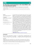
An example of a labelled dominance graph is
shown to the left of Fig. 1. Tree edges are drawn
as solid lines, and dominance edges as dotted lines,
directed from top to bottom. This graph can serve
as an USR for the sentence “a representative of
a company saw a sample” if we demand that the
holes are “plugged” by roots while realising the
dominance edges as dominance, as in the two con-
figurations (of five) shown to the right. These con-
figurations are trees that encode semantic represen-
tations of the sentence. We will freely read config-
urations as ground terms over the signature Σ.
2.1 Hypernormally connected graphs
Throughout this paper, we will only consider hy-
pernormally connected (hnc) dominance graphs.
Hnc graphs are equivalent to chain-connected
dominance constraints (Koller et al., 2003), and
are closely related to dominance nets (Niehren and
Thater, 2003). Fuchss et al. (2004) have presented
a corpus study that strongly suggests that all dom-
inance graphs that are generated by current large-
scale grammars are (or should be) hnc.
Technically, a graph G is hypernormally con-
nected iff each pair of nodes is connected by a sim-
ple hypernormal path in G. A hypernormal path
(Althaus et al., 2003) in G is a path in the undi-
rected version G

u
of G that does not use two dom-
inance edges that are incident to the same hole.
Hnc graphs have a number of very useful struc-
tural properties on which this paper rests. One
which is particularly relevant here is that we can
predict in which way different fragments can dom-
inate each other.
Definition 2. Let G be a hnc dominance graph. A
fragment F
1
in G is called a possible dominator
of another fragment F
2
in G iff it has exactly one
hole h which is connected to R(F
2
) by a simple hy-
410
a
y
sample
y
see
x,y
a
x
repr-of
x,z
a

z
comp
z
1 2 3
4 5 6
7
a
y
a
x
a
z
1
2
3
sample
y
see
x,y
repr-of
x,z
comp
z
a
y
a
x
sample
y
see

x,y
repr-of
x,z
a
z
comp
z
1
2
3
Figure 1: A dominance graph that represents the five readings of the sentence “a representative of a
company saw a sample” (left) and two of its five configurations.
{1,2,3,4,5,6,7} :1, h
1
→ {4},h
2
→ {2,3,5,6,7}
2,h
3
→ {1,4,5},h
4
→ {3,6,7}
3,h
5
→ {5},h
6
→ {1,2,4,5,7}
{2,3,5,6,7} :2,h
3
→ {5},h

4
→ {3,6,7}
3,h
5
→ {6},h
6
→ {2,5,7}
{3,6,7} :3,h
5
→ {6},h
6
→ {7}
{2,5,7} :2,h
3
→ {5},h
4
→ {7}
{1,4,5} :1,h
1
→ {4},h
2
→ {5}
{1,2,4,5,7} :1,h
1
→ {4},h
2
→ {2,5,7}
2,h
3
→ {1,4,5},h

4
→ {7}
Figure 2: The chart for the graph in Fig. 1.
pernormal path which doesn’t use R(F
1
). We write
ch(F
1
,F
2
) for this unique h.
Lemma 1 (Koller and Thater (2006)). Let F
1
, F
2
be fragments in a hnc dominance graph G. If there
is a configuration C of G in which R(F
1
) dominates
R(F
2
), then F
1
is a possible dominator of F
2
, and
in particular ch(F
1
,F
2

) dominates R(F
2
) in C.
By applying this rather abstract result, we can
derive a number of interesting facts about the ex-
ample graph in Fig. 1. The fragments 1, 2, and 3
are possible dominators of all other fragments (and
of each other), while the fragments 4 through 7
aren’t possible dominators of anything (they have
no holes); so 4 through 7 must be leaves in any con-
figuration of the graph. In addition, if fragment 2
dominates fragment 3 in any configuration, then in
particular the right hole of 2 will dominate the root
of 3; and so on.
2.2 Dominance charts
Below we will not work with dominance graphs
directly. Rather, we will use dominance charts
(Koller and Thater, 2005b) as our USRs: they are
more explicit USRs, which support a more fine-
grained deletion of reading sets than graphs.
A dominance chart for the graph G is a mapping
of weakly connected subgraphs of G to sets of
splits (see Fig. 2), which describe possible ways
of constructing configurations of the subgraph.
A subgraph G

is assigned one split for each
fragment F in G

which can be at the root of a

configuration of G

. If the graph is hnc, removing
F from the graph splits G

into a set of weakly
connected components (wccs), each of which is
connected to exactly one hole of F. We also record
the wccs, and the hole to which each wcc belongs,
in the split. In order to compute all configurations
represented by a split, we can first compute
recursively the configurations of each component;
then we plug each combination of these sub-
configurations into the appropriate holes of the
root fragment. We define the configurations asso-
ciated with a subgraph as the union over its splits,
and those of the entire chart as the configurations
associated with the complete graph.
Fig. 2 shows the dominance chart correspond-
ing to the graph in Fig. 1. The chart represents
exactly the configuration set of the graph, and is
minimal in the sense that every subgraph and ev-
ery split in the chart can be used in constructing
some configuration. Such charts can be computed
efficiently (Koller and Thater, 2005b) from a dom-
inance graph, and can also be used to compute the
configurations of a graph efficiently.
The example chart expresses that three frag-
ments can be at the root of a configuration of the
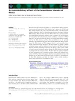
complete graph: 1, 2, and 3. The entry for the split

with root fragment 2 tells us that removing 2 splits
the graph into the subgraphs {1,4,5} and {3,6,7}
(see Fig. 3). If we configure these two subgraphs
recursively, we obtain the configurations shown in
the third column of Fig. 3; we can then plug these
sub-configurations into the appropriate holes of 2
and obtain a configuration for the entire graph.
Notice that charts can be exponentially larger
than the original graph, but they are still expo-
nentially smaller than the entire set of readings
because common subgraphs (such as the graph
{2,5,7} in the example) are represented only once,
411
1 2 3
4 5 6 7
h
2
h
1
h
4
h
3
h
6
h
5
1 3
4 5 6 7
h

2
h
1
h
6
h
5
→ →
1 3
4 5 6 7
2
1 3
4 5 6 7
→
Figure 3: Extracting a configuration from a chart.
and are small in practice (see (Koller and Thater,
2005b) for an analysis). Thus the chart can still
serve as an underspecified representation.
3 Equivalence
Now let’s define equivalence of readings more
precisely. Equivalence of semantic representations
is traditionally defined as the relation between
formulas (say, of first-order logic) which have
the same interpretation. However, even first-order
equivalence is an undecidable problem, and broad-
coverage semantic representations such as those
computed by the ERG usually have no well-
defined model-theoretic semantics and therefore
no concept of semantic equivalence.
On the other hand, we do not need to solve

the full semantic equivalence problem, as we only
want to compare formulas that are readings of the
same sentence, i.e. different configurations of the
same USR. Such formulas only differ in the way
that the fragments are combined. We can therefore
approximate equivalence by using a rewrite system
that permutes fragments and defining equivalence
of configurations as mutual rewritability as usual.
By way of example, consider again the two con-
figurations shown in Fig. 1. We can obtain the sec-
ond configuration from the (semantically equiva-
lent) first one by applying the following rewrite
rule, which rotates the fragments 1 and 2:
a
x
(a
z
(P,Q),R) → a
z
(P,a
x
(Q,R)) (3)
Thus we take these two configurations to be
equivalent with respect to the rewrite rule. (We
could also have argued that the second configura-
tion can be rewritten into the first by using the in-
verted rule.)
We formalise this rewriting-based notion of
equivalence as follows. The definition uses the ab-
breviation x

[1,k)
for the sequence x
1
, ,x
k−1
, and
x
(k,n]
for x
k+1
, ,x
n
.
Definition 3. A permutation system R is a system
of rewrite rules over the signature Σ of the follow-
ing form:
f
1
(x
[1,i)
, f
2
(y
[1,k)
,z,y
(k,m]
),x
(i,n]
) →
f

2
(y
[1,k)
, f
1
(x
[1,i)
,z,x
(i,n]
),y
(k,m]
)
The permutability relation P(R) is the binary rela-
tion P(R) ⊆ (Σ × N)
2
which contains exactly the
tuples (( f
1
,i),( f
2
,k)) and (( f
2
,k),( f
1
,i)) for each
such rewrite rule. Two terms are equivalent with re-
spect to R, s ≈
R
t, iff there is a sequence of rewrite
steps and inverse rewrite steps that rewrite s into t.

If G is a graph over Σ and R a permutation sys-
tem, then we write SC
R
(G) for the set of equiva-
lence classes Conf(G)/≈
R
, where Conf(G) is the
set of configurations of G.
The rewrite rule (3) above is an instance of this
schema, as are the other three permutations of ex-
istential quantifiers. These rules approximate clas-
sical semantic equivalence of first-order logic, as
they rewrite formulas into classically equivalent
ones. Indeed, all five configurations of the graph
in Fig. 1 are rewriting-equivalent to each other.
In the case of the semantic representations gen-
erated by the ERG, we don’t have access to an
underlying interpretation. But we can capture lin-
guistic intuitions about the equivalence of readings
in permutation rules. For instance, proper names
and pronouns (which the ERG analyses as scope-
bearers, although they can be reduced to constants
without scope) can be permuted with anything. In-
definites and definites permute with each other if
they occur in each other’s scope, but not if they
occur in each other’s restriction; and so on.
4 Redundancy elimination
Given a permutation system, we can now try to get
rid of readings that are equivalent to other readings.
One way to formalise this is to enumerate exactly

one representative of each equivalence class. How-
ever, after such a step we would be left with a col-
lection of semantic representations rather than an
USR, and could not use the USR for ruling out
further readings. Besides, a naive algorithm which
412
first enumerates all configurations would be pro-
hibitively slow.
We will instead tackle the following underspec-
ified redundancy elimination problem: Given an
USR G, compute an USR G

with Conf(G

) ⊆
Conf(G) and SC
R
(G) = SC
R
(G

). We want
Conf(G

) to be as small as possible. Ideally, it
would contain no two equivalent readings, but in
practice we won’t always achieve this kind of com-
pleteness. Our redundancy elimination algorithm
will operate on a dominance chart and successively
delete splits and subgraphs from the chart.

4.1 Permutable fragments
Because the algorithm must operate on USRs
rather than configurations, it needs a way to pre-
dict from the USR alone which fragments can be
permuted in configurations. This is not generally
possible in unrestricted graphs, but for hnc graphs
it is captured by the following criterion.
Definition 4. Let R be a permutation system. Two
fragments F
1
and F
2
with root labels f
1
and f
2
in a hnc graph G are called R-permutable iff
they are possible dominators of each other and
(( f
1
,ch(F
1
,F
2
)),( f
2
,ch(F
2
,F
1

))) ∈ P(R).
For example, in Fig. 1, the fragments 1 and 2
are permutable, and indeed they can be permuted
in any configuration in which one is the parent of
the other. This is true more generally:
Lemma 2 (Koller and Thater (2006)). Let G be a
hnc graph, F
1
and F
2
be R-permutable fragments
with root labels f
1
and f
2
, and C
1
any config-
uration of G of the form C( f
1
( , f
2
( ), ))
(where C is the context of the subterm). Then
C
1
can be R-rewritten into a tree C
2
of the form
C( f

2
( , f
1
( ), )) which is also a configura-
tion of G.
The proof uses the hn connectedness of G in two
ways: in order to ensure that C
2
is still a configu-
ration of G, and to make sure that F
2
is plugged
into the correct hole of F
1
for a rule application
(cf. Lemma 1). Note that C
2
≈
R
C
1
by definition.
4.2 The redundancy elimination algorithm
Now we can use permutability of fragments to
define eliminable splits. Intuitively, a split of a
subgraph G is eliminable if each of its configura-
tions is equivalent to a configuration of some other
split of G. Removing such a split from the chart
will rule out some configurations; but it does not
change the set of equivalence classes.

Definition 5. Let R be a permutation system. A
split S = (F, , h
i
→ G
i
, ) of a graph G is called
eliminable in a chart Ch if some G
i
contains a frag-
ment F

such that (a) Ch contains a split S

of G
with root fragment F

, and (b) F

is R-permutable
with F and all possible dominators of F

in G
i
.
In Fig. 1, each of the three splits is eliminable.
For example, the split with root fragment 1 is elim-
inable because the fragment 3 permutes both with
2 (which is the only possible dominator of 3 in the
same wcc) and with 1 itself.
Proposition 3. Let Ch be a dominance chart, and

let S be an eliminable split of a hnc subgraph. Then
SC(Ch) = SC(Ch −S).
Proof. Let C be an arbitrary configuration of S =
(F,h
1
→ G
1
, ,h
n
→ G
n
), and let F

∈ G
i
be the
root fragment of the assumed second split S

.
Let F
1
, ,F
n
be those fragments in C that are
properly dominated by F and properly dominate
F

. All of these fragments must be possible domi-
nators of F


, and all of them must be in G
i
as well,
so F

is permutable with each of them. F

must
also be permutable with F. This means that we can
apply Lemma 2 repeatedly to move F

to the root
of the configuration, obtaining a configuration of
S

which is equivalent to C.
Notice that we didn’t require that Ch must be
the complete chart of a dominance graph. This
means we can remove eliminable splits from a
chart repeatedly, i.e. we can apply the following
redundancy elimination algorithm:
REDUNDANCY-ELIMINATION(Ch, R)
1 for each split S in Ch
2 do if S is eliminable with respect to R
3 then remove S from Ch
Prop. 3 shows that the algorithm is a correct
algorithm for the underspecified redundancy
elimination problem. The particular order in
which eliminable splits are removed doesn’t
affect the correctness of the algorithm, but it may

change the number of remaining configurations.
The algorithm generalises an earlier elimination
algorithm (Koller and Thater, 2006) in that the
earlier algorithm required the existence of a single
split which could be used to establish eliminability
of all other splits of the same subgraph.
We can further optimise this algorithm by keep-
ing track of how often each subgraph is referenced
413
every
z
D
x,y,z
a
y
a
x
1 2 3
A
x
B
y
C
z
4 5 6
7
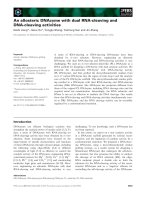
Figure 4: A graph for which the algorithm is not
complete.
by the splits in the chart. Once a reference count
drops to zero, we can remove the entry for this

subgraph and all of its splits from the chart. This
doesn’t change the set of configurations of the
chart, but may further reduce the chart size. The
overall runtime for the algorithm is O(n
2
S), where
S is the number of splits in Ch and n is the num-
ber of nodes in the graph. This is asymptotically
not much slower than the runtime O((n + m)S) it
takes to compute the chart in the first place (where
m is the number of edges in the graph).
4.3 Examples and discussion
Let’s look at a run of the algorithm on the chart
in Fig. 2. The algorithm can first delete the elim-
inable split with root 1 for the entire graph G. After
this deletion, the splits for G with root fragments
2 and 3 are still eliminable; so we can e.g. delete
the split for 3. At this point, only one split is left
for G. The last split for a subgraph can never be
eliminable, so we are finished with the splits for
G. This reduces the reference count of some sub-
graphs (e.g. {2,3,5,6,7}) to 0, so we can remove
these subgraphs too. The output of the algorithm is
the chart shown below, which represents a single
configuration (the one shown in Fig. 3).
{1,2,3,4,5,6,7} :2, h
2
→ {1,4},h
4
→ {3,6,7}

{1,4} :1,h
1
→ {4}
{3,6,7} :3,h
5
→ {6},h
6
→ {7}
In this case, the algorithm achieves complete re-
duction, in the sense that the final chart has no two
equivalent configurations. It remains complete for
all variations of the graph in Fig. 1 in which some
or all existential quantifiers are replaces by univer-
sal quantifiers. This is an improvement over our
earlier algorithm (Koller and Thater, 2006), which
computed a chart with four configurations for the
graph in which 1 and 2 are existential and 3 is uni-
versal, as opposed to the three equivalence classes
of this graph’s configurations.
However, the present algorithm still doesn’t
achieve complete reduction for all USRs. One ex-
ample is shown in Fig. 4. This graph has six config-
urations in four equivalence classes, but no split of
the whole graph is eliminable. The algorithm will
delete a split for the subgraph {1,2,4,5,7}, but the
final chart will still have five, rather than four, con-
figurations. A complete algorithm would have to
recognise that {1,3,4,6,7} and {2,3,5,6,7} have
splits (for 1 and 2, respectively) that lead to equiv-
alent configurations and delete one of them. But

it is far from obvious how such a non-local deci-
sion could be made efficiently, and we leave this
for future work.
5 Evaluation
In this final section, we evaluate the the effective-
ness and efficiency of the elimination algorithm:
We run it on USRs from a treebank and measure
how many readings are redundant, to what extent
the algorithm eliminates this redundancy, and how
much time it takes to do this.
Resources. The experiments are based on the
Rondane corpus, a Redwoods (Oepen et al., 2002)
style corpus which is distributed with the English
Resource Grammar (Flickinger, 2002). The cor-
pus contains analyses for 1076 sentences from the
tourism domain, which are associated with USRs
based upon Minimal Recursion Semantics (MRS).
The MRS representations are translated into dom-
inance graphs using the open-source utool tool
(Koller and Thater, 2005a), which is restricted to
MRS representations whose translations are hnc.
By restricting ourselves to such MRSs, we end up
with a data set of 999 dominance graphs. The aver-
age number of scope bearing operators in the data
set is 6.5, and the median number of readings is 56.
We then defined a (rather conservative) rewrite
system R
ERG
for capturing the permutability rela-
tion of the quantifiers in the ERG. This amounted

to 34 rule schemata, which are automatically ex-
panded to 494 rewrite rules.
Experiment: Reduction. We first analysed the
extent to which our algorithm eliminated the re-
dundancy of the USRs in the corpus. We com-
puted dominance charts for all USRs, ran the al-
gorithm on them, and counted the number of con-
figurations of the reduced charts. We then com-
pared these numbers against a baseline and an up-
per bound. The upper bound is the true number of
414
1
10
100
1000
10000
100000
0 1 2 3 4 5 6 7 8 9 10 11 12 13
log(#configurations)
Factor
Algorithm Baseline Classes
Figure 5: Mean reduction factor on Rondane.
equivalence classes with respect to R
ERG
; for effi-
ciency reasons we could only compute this num-
ber for USRs with up to 500.000 configurations
(95 % of the data set). The baseline is given by
the number of readings that remain if we replace
proper names and pronouns by constants and vari-

ables, respectively. This simple heuristic is easy to
compute, and still achieves nontrivial redundancy
elimination because proper names and pronouns
are quite frequent (28% of the noun phrase occur-
rences in the data set). It also shows the degree of
non-trivial scope ambiguity in the corpus.
For each measurement, we sorted the USRs ac-
cording to the number N of configurations, and
grouped USRs according to the natural logarithm
of N (rounded down) to obtain a logarithmic scale.
First, we measured the mean reduction factor
for each log(N) class, i.e. the ratio of the num-
ber of all configurations to the number of remain-
ing configurations after redundancy elimination
(Fig. 5). The upper-bound line in the figure shows
that there is a great deal of redundancy in the USRs
in the data set. The average performance of our
algorithm is close to the upper bound and much
0%
20%
40%
60%
80%
100%
0 1 2 3 4 5 6 7 8 9 10 11 12 13
log(#configurations)
Algorithm Baseline
Figure 6: Percentage of USRs for which the algo-
rithm and the baseline achieve complete reduction.
0

1
10
100
1000
10000
0 1 2 3 4 5 6 7 8 9 10 11 12 13
log(#configurations)
time (ms)
Full Chart Reduced Chart Enumeration
Figure 7: Mean runtimes.
better than the baseline. For USRs with fewer than
e
8
= 2980 configurations (83 % of the data set), the
mean reduction factor of our algorithm is above
86 % of the upper bound. The median number
of configurations for the USRs in the whole data
set is 56, and the median number of equivalence
classes is 3; again, the median number of config-
urations of the reduced charts is very close to the
upper bound, at 4 (baseline: 8). The highest reduc-
tion factor for an individual USR is 666.240.
We also measured the ratio of USRs for which
the algorithm achieves complete reduction (Fig. 6):
The algorithm is complete for 56 % of the USRs
in the data set. It is complete for 78 % of the USRs
with fewer than e
5
= 148 configurations (64 % of
the data set), and still complete for 66 % of the

USRs with fewer than e
8
configurations.
Experiment: Efficiency. Finally, we measured
the runtime of the elimination algorithm. The run-
time of the elimination algorithm is generally com-
parable to the runtime for computing the chart in
the first place. However, in our experiments we
used an optimised version of the elimination algo-
rithm, which computes the reduced chart directly
from a dominance graph by checking each split
for eliminability before it is added to the chart.
We compare the performance of this algorithm to
the baseline of computing the complete chart. For
comparison, we have also added the time it takes
to enumerate all configurations of the graph, as a
lower bound for any algorithm that computes the
equivalence classes based on the full set of config-
urations. Fig. 7 shows the mean runtimes for each
log(N) class, on the USRs with less than one mil-
lion configurations (958 USRs).
As the figure shows, the asymptotic runtimes
for computing the complete chart and the reduced
chart are about the same, whereas the time for
415
enumerating all configurations grows much faster.
(Note that the runtime is reported on a logarithmic
scale.) For USRs with many configurations, com-
puting the reduced chart actually takes less time
on average than computing the complete chart

because the chart-filling algorithm is called on
fewer subgraphs. While the reduced-chart algo-
rithm seems to be slower than the complete-chart
one for USRs with less than e
5
configurations,
these runtimes remain below 20 milliseconds on
average, and the measurements are thus quite un-
reliable. In summary, we can say that there is no
overhead for redundancy elimination in practice.
6 Conclusion
We presented an algorithm for redundancy elimina-
tion on underspecified chart representations. This
algorithm successively deletes eliminable splits
from the chart, which reduces the set of described
readings while making sure that at least one rep-
resentative of each original equivalence class re-
mains. Equivalence is defined with respect to a cer-
tain class of rewriting systems; this definition ap-
proximates semantic equivalence of the described
formulas and fits well with the underspecification
setting. The algorithm runs in polynomial time in
the size of the chart.
We then evaluated the algorithm on the Ron-
dane corpus and showed that it is useful in practice:
the median number of readings drops from 56 to
4, and the maximum individual reduction factor is
666.240. The algorithm achieves complete reduc-
tion for 56% of all sentences. It does this in neg-
ligible runtime; even the most difficult sentences

in the corpus are reduced in a matter of seconds,
whereas the enumeration of all readings would
take about a year. This is the first corpus evalua-
tion of a redundancy elimination in the literature.
The algorithm improves upon previous work
(Koller and Thater, 2006) in that it eliminates more
splits from the chart. It is an improvement over ear-
lier algorithms for enumerating irredundant read-
ings (Vestre, 1991; Chaves, 2003) in that it main-
tains underspecifiedness; note that these earlier pa-
pers never made any claims with respect to, or eval-
uated, completeness.
There are a number of directions in which the
present algorithm could be improved. We are cur-
rently pursuing some ideas on how to improve the
completeness of the algorithm further. It would
also be worthwhile to explore heuristics for the or-
der in which splits of the same subgraph are elim-
inated. The present work could be extended to al-
low equivalence with respect to arbitrary rewrite
systems. Most generally, we hope that the methods
developed here will be useful for defining other
elimination algorithms, which take e.g. full world
knowledge into account.
References
E. Althaus, D. Duchier, A. Koller, K. Mehlhorn, J. Niehren,
and S. Thiel. 2003. An efficient graph algorithm for dom-
inance constraints. Journal of Algorithms, 48:194–219.
P. Blackburn and J. Bos. 2005. Representation and Inference
for Natural Language. A First Course in Computational

Semantics. CSLI Publications.
R. P. Chaves. 2003. Non-redundant scope disambiguation
in underspecified semantics. In Proc. 8th ESSLLI Student
Session.
A. Copestake, D. Flickinger, C. Pollard, and I. Sag. 2004.
Minimal recursion semantics: An introduction. Journal of
Language and Computation. To appear.
M. Egg, A. Koller, and J. Niehren. 2001. The Constraint
Language for Lambda Structures. Logic, Language, and
Information, 10.
D. Flickinger. 2002. On building a more efficient grammar
by exploiting types. In J. Tsujii S. Oepen, D. Flickinger
and H. Uszkoreit, editors, Collaborative Language Engi-
neering. CSLI Publications, Stanford.
R. Fuchss, A. Koller, J. Niehren, and S. Thater. 2004. Mini-
mal recursion semantics as dominance constraints: Trans-
lation, evaluation, and analysis. In Proc. of the 42nd ACL.
A. Koller and S. Thater. 2005a. Efficient solv ing and ex-
ploration of scope ambiguities. In ACL-05 Demonstration
Notes, Ann Arbor.
A. Koller and S. Thater. 2005b. The evolution of dominance
constraint solvers. In Proceedings of the ACL-05 Work-
shop on Software, Ann Arbor.
A. Koller and S. Thater. 2006. Towards a redundancy elimi-
nation algorithm for underspecified descriptions. In Proc.
5th Intl. Workshop on Inference in Computational Seman-
tics (ICoS-5).
A. Koller, J. Niehren, and S. Thater. 2003. Bridging the gap
between underspecification formalisms: Hole semantics as
dominance constraints. In Proc. 10th EACL.

J. Niehren and S. Thater. 2003. Bridging the gap between
underspecification formalisms: Minimal recursion seman-
tics as dominance constraints. In Proc. of the 41st ACL.
S. Oepen, K. Toutanova, S. Shieber, C. Manning,
D. Flickinger, and T. Brants. 2002. The LinGO Red-
woods treebank: Motivation and preliminary applications.
In Proceedings of COLING’02.
K. van Deemter and S. Peters. 1996. Semantic Ambiguity
and Underspecification. CSLI, Stanford.
E. Vestre. 1991. An algorithm for generating non-redundant
quantifier scopings. In Proc. of the Fifth EACL, Berlin.
416