Application of ROMS-SWAN coupled model to simulate hydrodynamic field in Hai Phong
Bạn đang xem bản rút gọn của tài liệu. Xem và tải ngay bản đầy đủ của tài liệu tại đây (5.26 MB, 10 trang )
Vietnam Journal of Marine Science and Technology 2022, 22(2) 123–132
Vietnam Academy of Science and Technology
Vietnam Journal of Marine Science and Technology
journal homepage: vjs.ac.vn/index.php/jmst
Application of ROMS-SWAN coupled model to simulate hydrodynamic
field in Hai Phong
Nguyen Le Tuan*, Nguyen Thi Khang, Le Duc Dung, Nguyen Hoang Anh
Vietnam Institute of Seas and Islands, Hanoi, Vietnam
*
E-mail:
Received: 7 June 2021; Accepted: 15 October 2021
ABSTRACT
ROMS and SWAN models have been used quite commonly in studying hydrodynamics. These are opensource models which are suitable for development research. However, using the ROMS-SWAN coupled
model has not been studied and applied much in Vietnam. This paper presents the study and use of the
ROMS-SWAN coupled model in the COAWST system to calculate the hydrodynamic field in Hai Phong at
a primitive level. The calculation gives quite good results when compared with the measured data. The
results of this study are the basis for the application of the COAWST model system to calculate sediment
transport.
Keywords: Coupled model, ROMS, SWAN, hydrodynamics.
Citation: Nguyen Le Tuan, Nguyen Thi Khang, Le Duc Dung, and Nguyen Hoang Anh, 2022. Application of ROMSSWAN coupled model to simulate hydrodynamic field in Hai Phong. Vietnam Journal of Marine Science and
Technology, 22(2), 123–132. />ISSN 1859-3097/© 2022 Vietnam Academy of Science and Technology (VAST)
123
Nguyen Le Tuan et al./Vietnam Journal of Marine Science and Technology 2022, 22(2) 123–132
INTRODUCTION
With the vigorous development of
computer science, numerical models are
increasingly developed and widely used. There
are two models used to compute processes in
the seas and oceans: commercial models and
open-source models. Commercial models have
the advantage of running because they have
been calibrated and tested and have an intuitive
and easy-to-use interface. Still, the cost of these
models is relatively high; users cannot update
the results of new research into the model, are
unable to develop applications in their
direction, and it is not easy to link with other
models. Meanwhile, open-source models are
usually free; users can continuously improve
them according to their research direction and
link to other open-source models. However,
these models often make it more difficult for
users because they do not have an interface,
and users also need a detailed understanding of
programming. That leads to which model to use
depending on each author’s purpose.
Figure 1. Study area
Understanding the importance of the
interactions between the sea and the
atmosphere, the USGS has been leading the
development of a Coupled Ocean-AtmosphereWaves-Sediment
Transport
(COAWST)
Modeling System. The COAWST modeling
system joins an ocean model, an atmosphere
model, a wave model, and a sediment transport
model for studies of coastal change. The
COAWST Modeling System includes an ocean
component—Regional Ocean Modeling System
(ROMS) [1]; atmosphere component—Weather
Research and Forecast Model (WRF),
hydrology component- WRF_Hydro; wave
components—Simulating Waves Nearshore
124
(SWAN) [2], WAVEWATCHIII, and InWave;
a sediment component—the USGS Community
Sediment Models; and a sea ice model [3–5].
The model system allows calculation and
simulation by each model separately or
simultaneously many models.
In this study, the ROMS-SWAN coupled
model belonging to the COAWST system was
studied and used to simulate the hydrodynamic
field in Hai Phong. Usually, when using
separate models, the results from one model
can be used as input to another model;
however, these results need to be processed to
get the required format of the model. With the
COAWST system, users can use multiple
Nguyen Le Tuan et al./Vietnam Journal of Marine Science and Technology 2022, 22(2) 123–132
models simultaneously; the models use the
results of other models in the system as input
without the need for preprocessing steps like
when using separate models. The ROMS model
provides the SWAN model’s water level,
bathymetry, and current for. In contrast, the
SWAN model provides the ROMS model’s
wave parameters and radiation stress. Model
Coupling Toolkit (MCT [6]) was used to
coupled ROMS and SWAN [4].
DATA AND METHODS
Data
Bathymetry: The model can use ETOPO1
terrain data and GEBCO data. These data are
freely available to the user community in the
world. However, the accuracy of this data
source is not good, especially for shallow
water, coastal areas, and islands. For the sake
of relative detail, the data used in this study is a
combination of naval data of 1/25,000 scale,
naval data of 1/10,000 scale, and measured data
provided by project TNMT.2018.06.15.
Initial condition and boundary condition:
These data were obtained from the HYCOM
database ( />
HYCOM provides global data with a spatial
resolution of 0.125 degrees, 40 layers, and 3 h
temporal resolution [7].
In the model system, the forces are
obtained from the reanalysis database of the
European Centre for Medium-Range Weather
Forecasts. This database provides sea surface
forcing with a spatial resolution of 0.125
degrees and 3 h temporal resolution. The
effects used in the model include wind velocity
(U, V) at 10 m above sea level, longwave
radiation (lwrad), short wave radiation (sward),
air temperature (Tair), sea surface pressure
(Pair), sea surface precipitation, sea surface air
humidity (Qair).
Tide data. The liquid boundary condition is
given by the harmonic constituents of 14 waves
(M2, S2, K1, O1, N2, P1, K2, Q1, MF, MM,
M4, N4, MS4, MN4) taken from the global tidal
model [8].
This study uses the measured water level,
wave, and current data provided from the
project TNMT.2018.06.15 are used for model
calibration and verification. The location and
time of the survey are shown in Table 1 and
Figure 2.
Table 1. Location and time for measuring water level, waves, current
Time
2/8/2019–16/8/2019
25/4/2020–9/5/2020
Water level
Longitude
Latitude
106o50’50”E
20o47’54,6”N
106o50’50”E
20o47’54,6”N
Waves, current
Longitude
Latitude
106o58’19,37”E
20o34’39,24”N
106o58’19,54”E
20o35’30,31”N
Figure 2. Location of measuring stations
125
Nguyen Le Tuan et al./Vietnam Journal of Marine Science and Technology 2022, 22(2) 123–132
Methods
Implementation steps include preparing
data, creating a grid, calibrating and validating
the model, and calculating according to
scenarios.
There are quite a few tools to create grids
for ROMS models, such as Gridgen, Easygrid,
Gridbuilder, or tools written in Matlab such as
create_roms_xygrid.m,… in this study,
Gridbuilder was used due to its convenience
and visualization. Gridbuilder is an addon on
Matlab with its convenient interface, which can
create mesh files and bathymetry files for the
SWAN model [9].
After creating the mesh, using the
“editmask.m” program provided with the
model tools system to edit the mesh with
shoreline
data
taken
from
GSHHS
[10]. The mesh file for
the calculation will be received after updating
and smoothing the bathymetry.
For the SWAN model, there are many ways
to create a mesh for this model, but the most
convenient for the integrated model is to use the
same mesh as the ROMS model, with the
modeling system providing accompanying tools.
Using the command “roms2swan(‘grid.nc’)” on
Matlab will create a coordinate file
“swan_coord.grd” and a bathymetry file
“swan_bathy.bot” for SWAN model [11].
The data on boundary conditions, initial
conditions, impact forces, and tides are
obtained from HYCOM, ECMWF, and global
tidal models through scripts built on Matlab.
In this study, river influence is not considered,
and discharge/flow boundary conditions are
set to zero.
Calibrate and validate the model to
determine the model’s parameters suitable for
the research area. Nash coefficient (F2) and
correlation coefficient (R2) is used to evaluate
the calculated results with measured data.
After determining the parameters suitable
for the study area, calculations are carried out
according to the scenarios of Northeast monsoon
season and Southwest monsoon season.
RESULTS
Domains and grids
The calculation domain is shown in Fig. 3.
Calculation uses a grid with a resolution of
300 m × 300 m corresponding to 545 × 730
grid cells.
Figure 3. Calculation domain
Calibration and verification
Figure 4 compares the measured water
level data and the calculated results from the
126
model according to the modified parameters.
Looking at Figure 4, we can see the similarity
in phase and magnitude between the measured
Nguyen Le Tuan et al./Vietnam Journal of Marine Science and Technology 2022, 22(2) 123–132
data and the calculated results. Nash coefficient
(F2) is estimated to evaluate the accuracy of the
results from the model compared to the
measurement, the result F2 = 0.93. The F2 value
is relatively high, greater than 0.8, along with
the correlation coefficient R2 = 0.969 (Figure 5)
to ensure the exact conditions of the model.
Figure 4. Comparison of measured water level
data with calculated results
have similarities in phase and magnitude. Nash
coefficient is calculated for the value F2 = 0.83,
correlation coefficient R2 = 0.792 (Figure 7) to
ensure the reliability of the model.
Figure 7. Correlation of measured wave heights
and calculated results
The model calibration process gives quite
good results, shown in the similarity of phase
and magnitude and the value of the Nash
coefficient and the correlation coefficient are
relatively large. Thus, the model’s parameter
after calibration is suitable for the study area and
this parameter is used to validate the model.
Figure 5. Correlation of measured water level
and calculation results
Figure 8. Comparison of measured water level
data with calculated results
Figure 6. Comparison of wave height data
measured and calculated results
A comparison of the measured wave height
data and the calculated results from the model
according to the changed parameters is
presented in Figure 6. Looking at the figure, the
correlation between the measured data and the
calculated results can be seen; these values
Figure 9. Correlation of measured water level
and calculation results
127
Nguyen Le Tuan et al./Vietnam Journal of Marine Science and Technology 2022, 22(2) 123–132
Figure 10. Comparison of wave height data
measured and calculated results
Figure 11. Correlation of measured wave
heights and calculated results
Figure 12. Comparison of U flow velocity
components measured and
calculated results
Figure 13. Correlation of U flow velocity
components measured and
calculated results
128
Figure 14. Comparison of V flow velocity
components measured and
calculated results
Figure 15. Correlation of V flow velocity
components measured and calculated results
Figures 8–15 show the comparison between
actual measured water level, wave, and current
data with the calculated results from the
calibrated model and the correlation between
these data. These figures show the similarity in
phase and magnitude between these values. The
calculated correlation coefficients are all
greater than 0.65, so the model parameters
defined in the model are suitable for the
research area and can be used for other research
cases other.
Calculation scenario
In this study, the calculation is carried out
according to two regular monsoon seasons,
namely the Northeast monsoon season and the
Southwest monsoon season. Based on the data
collected over the above calculation time, the
statistical results of multi-year wave heights
(1979–2019) in the directions are shown in
Figure 16a for scenario 1 (Northeast monsoon
season) and Figure 16b for scenario 2
(Southwest monsoon season).
Statistics of multi-year wave data in the
calculated area show that NE and E are the two
Nguyen Le Tuan et al./Vietnam Journal of Marine Science and Technology 2022, 22(2) 123–132
dominant direction waves in the Northeast
monsoon season (scenario 1), and S and SE are
the two main direction waves in the Southwest
monsoon season (scenario 2).
Figure 16. Wave rose: a) Northeast monsoon; b) Southwest monsoon
Result
In the Northeast monsoon period (scenario 1),
with the input wave being NE and E direction,
the wave field calculation results show that the
wave propagating into the coastal area has
changed direction due to the barrier island; the
wave changes from NE and E direction to E
and ESE direction when entering the coastal
zone.
During the Southwest monsoon period
(scenario 2), because the input wave direction
is nearly perpendicular to the shoreline, there is
no offshore obstacle terrain, so the wave almost
does not change direction when entering the
coastal area. Waves propagating from offshore
to coastal areas are in S and SE directions.
Wave height decreases behind the islands, and
wave height in the coastal area is small (Fig. 17).
Figure 17. Detailed wave heights in the study area (scenario 1 (a) and scenario 2 (b))
129
Nguyen Le Tuan et al./Vietnam Journal of Marine Science and Technology 2022, 22(2) 123–132
a) Flood tide in spring tide
b) Flood tide in neap tide
c) Ebb tide in spring tide
d) Ebb tide in neap tide
Figure 18. Detailed currents field in the study area under scenario 1
a) Flood tide in spring tide
b) Flood tide in neap tide
c) Ebb tide in spring tide
d) Ebb tide in neap tide
Figure 19. Detailed currents field in the study area under scenario 2
130
Nguyen Le Tuan et al./Vietnam Journal of Marine Science and Technology 2022, 22(2) 123–132
During the Northeast monsoon period, the
current regime in this area is quite simple;
the current composition is mainly tidal
current, currents caused by waves are not
large. Figure 18 shows the current picture in
the Hai Phong area according to flood tide in
spring tide, flood tide in the neap tide, ebb
tide in spring tide, and ebb tide in the neap
tide. It is easy to see that the current
velocities are small during neap tide and
larger during spring tide due to the difference
in tidal oscillation amplitudes. The flow is
northeast in the flood tide and Southwest in
the ebb tide in the outer area; in the coastal
zone, the current tends to be perpendicular to
the flood tide and from the shore to the sea in
the ebb tide. Current velocities are typical in
the range of 10–50 cm/s and are mainly high
in the straits between islands.
Similar to the results in scenario 1, since
wave-induced currents are weak, tidal currents
are dominant, so the flow direction is identical
to scenario 2 (Fig. 19) is identical to scenario 1.
The flow is Northeast in the flood tide and
Southwest in the ebb tide in the outer area. In
the coastal area, the flow tends to be
perpendicular to the shore during the flood tide
and from the shore to the sea into the ebb tide.
The current velocity is small in the neap tide
and more extensive in the spring.
CONCLUSIONS AND RECOMMENDATIONS
The study has successfully applied the
ROMS-SWAN coupled model of the
COAWST
model
to
calculate
the
hydrodynamic field in Hai Phong. The
evaluation with measured data shows that the
ROMS-SWAN
coupled
model
system
simulates the hydrodynamic field quite well
with parallel calculation capabilities. This
system can meet the requirements for
hydrodynamic simulation in places with
dominant tides.
The wave and current field results
according to this calculation are relatively
simple. The calculation time is in the periods of
the Northeast monsoon season and the
Southwest monsoon season. However, this sea
area is located in the Gulf of Tonkin and is
relatively closed, so the wave height is
relatively small, and the sea is quite calm. In
the study, the influence of the river has not
been taken into the simulation; therefore, tidal
flow dominates during the entire calculation
period. This report is the first study using the
integrated model, so the obtained results are for
reference only. It is necessary to have more
comparative evaluation studies with each
component model, taking into account the
effects of the river, combined with the
meteorological model to evaluate the ability
and effectiveness of this model.
Acknowledgments: The authors would like to
thank the project TNMT.2018.06.15 for
supporting this study.
REFERENCES
[1] Technical
Documentation
ROMS
/>Ocean_Modeling_System_(ROMS),
accessed November 5, 2020.
[2] Scientific and technical documentation
SWAN />online_doc/swantech/swantech.html,
accessed November 5, 2020.
[3] USGS, COAWST: A Coupled-OceanAtmosphere-Wave-Sediment Transport
Modeling
System
/>ence/coawst-a-coupled-oceanatmosphere-wave-sediment-transportmodeling-system, accessed May 6, 2020.
[4] Warner, J. C., Armstrong, B., He, R., and
Zambon, J. B., 2010. Development of a
coupled
ocean–atmosphere–wave–
sediment transport (COAWST) modeling
system. Ocean modelling, 35(3), 230–
244. doi: 10.1016/ j.ocemod.2010.07.010
[5] Warner, J. C., Sherwood, C. R., Signell,
R. P., Harris, C. K., and Arango, H. G.,
2008. Development of a threedimensional, regional, coupled wave,
current, and sediment-transport model.
Computers & Geosciences, 34(10), 1284–
1306. doi: 10.1016/ j.cageo.2008.02.012
[6] Larson, J. W., Jacob, R. L., Ong, E., and
Loy, R., 2010. The Model Coupling
Toolkit API Reference Manual: MCT v.
131
Nguyen Le Tuan et al./Vietnam Journal of Marine Science and Technology 2022, 22(2) 123–132
[7]
[8]
132
2.10. Mathematics and Computer Science
Division, Argonne National Laboratory,
the USA.
HYCOM
consortium,
/>accessed November 6, 2020
Egbert & Erofeeva, OSU, 2010.
/>accessed
November 6, 2020.
[9]
Charles James, 2016, Gridbuilder
Instructions, 28 p.
[10] Paul Wessel, Walter H. F. Smith,
/>accessed
November 2, 2020
[11] USGS, 2020. COAWST User’s Manual,
Version 3.6, 91 p.