Báo cáo khoa học: "A Hierarchical Bayesian Language Model based on Pitman-Yor Processes" docx

Proceedings of the 21st International Conference on Computational Linguistics and 44th Annual Meeting of the ACL, pages 985–992,
Sydney, July 2006.
c
2006 Association for Computational Linguistics
A Hierarchical Bayesian Language Model based on Pitman-Yor Processes
Yee Whye Teh
School of Computing,
National University of Singapore,
3 Science Drive 2, Singapore 117543.

Abstract
We propose a new hierarchical Bayesian
n-gram model of natural languages. Our
model makes use of a generalization of
the commonly used Dirichlet distributions
called Pitman-Yor processes which pro-
duce power-law distributions more closely
resembling those in natural languages. We
show that an approximation to the hier-
archical Pitman-Yor language model re-
covers the exact formulation of interpo-
lated Kneser-Ney, one of the best smooth-
ing methods for n-gram language models.
Experiments verify that our model gives
cross entropy results superior to interpo-
lated Kneser-Ney and comparable to mod-
ified Kneser-Ney.
1 Introduction
Probabilistic language models are used exten-
sively in a variety of linguistic applications, in-
cluding speech recognition, handwriting recogni-

tion, optical character recognition, and machine
translation. Most language models fall into the
class of n-gram models, which approximate the
distribution over sentences using the conditional
distribution of each word given a context consist-
ing of only the previous n − 1 words,
P (sentence) ≈
T

i=1
P (word
i
| word
i−1
i−n+1
) (1)
with n = 3 (trigram models) being typical. Even
for such a modest value of n the number of param-
eters is still tremendous due to the large vocabu-
lary size. As a result direct maximum-likelihood
parameter fitting severely overfits to the training
data, and smoothing methods are indispensible for
proper training of n-gram models.
A large number of smoothing methods have
been proposed in the literature (see (Chen and
Goodman, 1998; Goodman, 2001; Rosenfeld,
2000) for good overviews). Most methods take a
rather ad hoc approach, where n-gram probabili-
ties for various values of n are combined together,
using either interpolation or back-off schemes.

Though some of these methods are intuitively ap-
pealing, the main justification has always been
empirical—better perplexities or error rates on test
data. Though arguably this should be the only
real justification, it only answers the question of
whether a method performs better, not how nor
why it performs better. This is unavoidable given
that most of these methods are not based on in-
ternally coherent Bayesian probabilistic models,
which have explicitly declared prior assumptions
and whose merits can be argued in terms of how
closely these fit in with the known properties of
natural languages. Bayesian probabilistic mod-
els also have additional advantages—it is rela-
tively straightforward to improve these models by
incorporating additional knowledge sources and
to include them in larger models in a principled
manner. Unfortunately the performance of pre-
viously proposed Bayesian language models had
been dismal compared to other smoothing meth-
ods (Nadas, 1984; MacKay and Peto, 1994).
In this paper, we propose a novel language
model based on a hierarchical Bayesian model
(Gelman et al., 1995) where each hidden variable
is distributed according to a Pitman-Yor process, a
nonparametric generalization of the Dirichlet dis-
tribution that is widely studied in the statistics and
probability theory communities (Pitman and Yor,
1997; Ishwaran and James, 2001; Pitman, 2002).
985

Our model is a direct generalization of the hierar-
chical Dirichlet language model of (MacKay and
Peto, 1994). Inference in our model is however
not as straightforward and we propose an efficient
Markov chain Monte Carlo sampling scheme.
Pitman-Yor processes produce power-law dis-
tributions that more closely resemble those seen
in natural languages, and it has been argued that
as a result they are more suited to applications
in natural language processing (Goldwater et al.,
2006). Weshow experimentally that our hierarchi-
cal Pitman-Yor language model does indeed pro-
duce results superior to interpolated Kneser-Ney
and comparable to modified Kneser-Ney, two of
the currently best performing smoothing methods
(Chen and Goodman, 1998). In fact we show a
stronger result—that interpolated Kneser-Ney can
be interpreted as a particular approximate infer-
ence scheme in the hierarchical Pitman-Yor lan-
guage model. Our interpretation is more useful
than past interpretations involving marginal con-
straints (Kneser and Ney, 1995; Chen and Good-
man, 1998) or maximum-entropy models (Good-
man, 2004) as it can recover the exact formulation
of interpolated Kneser-Ney, and actually produces
superior results. (Goldwater et al., 2006) has inde-
pendently noted the correspondence between the
hierarchical Pitman-Yor language model and in-
terpolated Kneser-Ney, and conjectured improved
performance in the hierarchical Pitman-Yor lan-

guage model, which we verify here.
Thus the contributions of this paper are three-
fold: in proposing a langauge model with excel-
lent performance and the accompanying advan-
tages of Bayesian probabilistic models, in propos-
ing a novel and efficient inference scheme for the
model, and in establishing the direct correspon-
dence between interpolated Kneser-Ney and the
Bayesian approach.
We describe the Pitman-Yor process in Sec-
tion 2, and propose the hierarchical Pitman-Yor
language model in Section 3. In Sections 4 and
5 we give a high level description of our sampling
based inference scheme, leaving the details to a
technical report (Teh, 2006). We also show how
interpolated Kneser-Ney can be interpreted as ap-
proximate inference in the model. We show ex-
perimental comparisons to interpolated and mod-
ified Kneser-Ney, and the hierarchical Dirichlet
language model in Section 6 and conclude in Sec-
tion 7.
2 Pitman-Yor Process
Pitman-Yor processes are examples of nonpara-
metric Bayesian models. Here we give a quick de-
scription of the Pitman-Yor process in the context
of a unigram language model; good tutorials on
such models are provided in (Ghahramani, 2005;
Jordan, 2005). Let W be a fixed and finite vocabu-
lary of V words. For each word w ∈ W let G(w)
be the (to be estimated) probability of w, and let

G = [G(w)]
w∈W
be the vector of word probabili-
ties. We place a Pitman-Yor process prior on G:
G ∼ PY(d, θ, G
0
) (2)
where the three parameters are: a discount param-
eter 0 ≤ d < 1, a strength parameter θ > −d and
a mean vector G
0
= [G
0
(w)]
w∈W
. G
0
(w) is the
a priori probability of word w: before observing
any data, we believe word w should occur with
probability G
0
(w). In practice this is usually set
uniformly G
0
(w) = 1/V for all w ∈ W . Both θ
and d can be understood as controlling the amount
of variability around G
0
in different ways. When

d = 0 the Pitman-Yor process reduces to a Dirich-
let distribution with parameters θG
0
.
There is in general no known analytic form for
the density of PY(d, θ, G
0
) when the vocabulary
is finite. However this need not deter us as we
will instead work with the distribution over se-
quences of words induced by the Pitman-Yor pro-
cess, which has a nice tractable form and is suffi-
cient for our purpose of language modelling. To
be precise, notice that we can treat both G and
G
0
as distributions over W , where word w ∈ W
has probability G(w) (respectively G
0
(w)). Let
x
1
, x
2
, . . . be a sequence of words drawn inde-
pendently and identically (i.i.d.) from G. We
shall describe the Pitman-Yor process in terms of
a generative procedure that produces x
1
, x

2
, . . . it-
eratively with G marginalized out. This can be
achieved by relating x
1
, x
2
, . . . to a separate se-
quence of i.i.d. draws y
1
, y
2
, . . . from the mean
distribution G
0
as follows. The first word x
1
is
assigned the value of the first draw y
1
from G
0
.
Let t be the current number of draws from G
0
(currently t = 1), c
k
be the number of words as-
signed the value of draw y
k

(currently c
1
= 1),
and c
·
=

t
k=1
c
k
be the current number of draws
from G. For each subsequent word x
c
·
+1
, we ei-
ther assign it the value of a previous draw y
k
with
probability
c
k
−d
θ+c
·
(increment c
k
; set x
c

·
+1
← y
k
),
or we assign it the value of a new draw from G
0
986
10
0
10
1
10
2
10
3
10
4
10
5
10
6
10
0
10
1
10
2
10
3

10
4
10
5
10
0
10
1
10
2
10
3
10
4
10
5
10
6
10
0
10
1
10
2
10
3
10
4
10
5

10
0
10
1
10
2
10
3
10
4
10
5
10
6
0
0.2
0.4
0.6
0.8
1
10
0
10
1
10
2
10
3
10
4

10
5
10
6
0
0.2
0.4
0.6
0.8
1
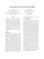
Figure 1: First panel: number of unique words as a function of the number of words drawn on a log-log
scale, with d = .5 and θ = 1 (bottom), 10 (middle) and 100 (top). Second panel: same, with θ = 10
and d = 0 (bottom), .5 (middle) and .9 (top). Third panel: proportion of words appearing only once, as
a function of the number of words drawn, with d = .5 and θ = 1 (bottom), 10 (middle), 100 (top). Last
panel: same, with θ = 10 and d = 0 (bottom), .5 (middle) and .9 (top).
with probability
θ+dt
θ+c
·
(increment t; set c
t
= 1;
draw y
t
∼ G
0
; set x
c
·
+1

← y
t
).
The above generative procedure produces a se-
quence of words drawn i.i.d. from G, with G
marginalized out. It is informative to study the
Pitman-Yor process in terms of the behaviour it
induces on this sequence of words. Firstly, no-
tice the rich-gets-richer clustering property: the
more words have been assigned to a draw from
G
0
, the more likely subsequent words will be as-
signed to the draw. Secondly, the more we draw
from G
0
, the more likely a new word will be as-
signed to a new draw from G
0
. These two ef-
fects together produce a power-law distribution
where many unique words are observed, most of
them rarely. In particular, for a vocabulary of un-
bounded size and for d > 0, the number of unique
words scales as O(θT
d
) where T is the total num-
ber of words. For d = 0, we have a Dirichlet dis-
tribution and the number of unique words grows
more slowly at O(θ log T).

Figure 1 demonstrates the power-law behaviour
of the Pitman-Yor process and how this depends
on d and θ. In the first two panels we show the
average number of unique words among 10 se-
quences of T words drawn from G, as a func-
tion of T , for various values of θ and d. We
see that θ controls the overall number of unique
words, while d controls the asymptotic growth of
the number of unique words. In the last two pan-
els, we show the proportion of words appearing
only once among the unique words; this gives an
indication of the proportion of words that occur
rarely. We see that the asymptotic behaviour de-
pends on d but not on θ, with larger d’s producing
more rare words.
This procedure for generating words drawn
from G is often referred to as the Chinese restau-
rant process (Pitman, 2002). The metaphor is as
follows. Consider a sequence of customers (cor-
responding to the words draws from G) visiting a
Chinese restaurant with an unbounded number of
tables (corresponding to the draws from G
0
), each
of which can accommodate an unbounded number
of customers. The first customer sits at the first ta-
ble, and each subsequent customer either joins an
already occupied table (assign the word to the cor-
responding draw from G
0

), or sits at a new table
(assign the word to a new draw from G
0
).
3 Hierarchical Pitman-Yor Language
Models
We describe an n-gram language model based on a
hierarchical extension of the Pitman-Yor process.
An n-gram language model defines probabilities
over the current word given various contexts con-
sisting of up to n − 1 words. Given a context u,
let G
u
(w) be the probability of the current word
taking on value w. We use a Pitman-Yor process
as the prior for G
u
[G
u
(w)]
w∈W
, in particular,
G
u
∼ PY(d
|u|
, θ
|u|
, G
π(u)

) (3)
where π(u) is the suffix of u consisting of all but
the earliest word. The strength and discount pa-
rameters are functions of the length |u| of the con-
text, while the mean vector is G
π(u)
, the vector
of probabilities of the current word given all but
the earliest word in the context. Since we do not
know G
π(u)
either, We recursively place a prior
over G
π(u)
using (3), but now with parameters
θ
|π(u)|
, d
|π(u)|
and mean vector G
π(π(u))
instead.
This is repeated until we get to G
∅
, the vector
of probabilities over the current word given the
987
empty context ∅. Finally we place a prior on G
∅
:

G
∅
∼ PY(d
0
, θ
0
, G
0
) (4)
where G
0
is the global mean vector, given a uni-
form value of G
0
(w) = 1/V for all w ∈ W . Fi-
nally, we place a uniform prior on the discount pa-
rameters and a Gamma(1, 1) prior on the strength
parameters. The total number of parameters in the
model is 2n.
The structure of the prior is that of a suffix tree
of depth n, where each node corresponds to a con-
text consisting of up to n−1 words, and each child
corresponds to adding a different word to the be-
ginning of the context. This choice of the prior
structure expresses our belief that words appearing
earlier in a context have (a priori) the least impor-
tance in modelling the probability of the current
word, which is why they are dropped first at suc-
cessively higher levels of the model.
4 Hierarchical Chinese Restaurant

Processes
We describe a generative procedure analogous
to the Chinese restaurant process of Section 2
for drawing words from the hierarchical Pitman-
Yor language model with all G
u
’s marginalized
out. This gives us an alternative representation of
the hierarchical Pitman-Yor language model that
is amenable to efficient inference using Markov
chain Monte Carlo sampling and easy computa-
tion of the predictive probabilities for test words.
The correspondence between interpolated Kneser-
Ney and the hierarchical Pitman-Yor language
model is also apparent in this representation.
Again we may treat each G
u
as a distribution
over the current word. The basic observation is
that since G
u
is Pitman-Yor process distributed,
we can draw words from it using the Chinese
restaurant process given in Section 2. Further, the
only operation we need of its parent distribution
G
π(u)
is to draw words from it too. Since G
π(u)
is itself distributed according to a Pitman-Yor pro-

cess, we can use another Chinese restaurant pro-
cess to draw words from that. This is recursively
applied until we need draws from the global mean
distribution G
0
, which is easy since it is just uni-
form. We refer to this as the hierarchical Chinese
restaurant process.
Let us introduce some notations. For each con-
text u we have a sequence of words x
u1
, x
u2
, . . .
drawn i.i.d. from G
u
and another sequence of
words y
u1
, y
u2
, . . . drawn i.i.d. from the parent
distribution G
π(u)
. We use l to index draws from
G
u
and k to index the draws from G
π(u)
. Define

t
uw k
= 1 if y
uk
takes on value w, and t
uw k
= 0
otherwise. Each word x
ul
is assigned to one of
the draws y
uk
from G
π(u)
. If y
uk
takes on value
w define c
uw k
as the number of words x
ul
drawn
from G
u
assigned to y
uk
, otherwise let c
uw k
= 0.
Finally we denote marginal counts by dots. For

example, c
u·k
is the number of x
ul
’s assigned the
value of y
uk
, c
uw·
is the number of x
ul
’s with
value w, and t
u··
is the current number of draws
y
uk
from G
π(u)
. Notice that we have the follow-
ing relationships among the c
uw·
’s and t
uw·
:

t
uw·
= 0 if c
uw·

= 0;
1 ≤ t
uw·
≤ c
uw·
if c
uw·
> 0;
(5)
c
uw·
=

u

:π(u

)=u
t
u

w·
(6)
Pseudo-code for drawing words using the hier-
archical Chinese restaurant process is given as a
recursive function DrawWord(u), while pseudo-
code for computing the probability that the next
word drawn from G
u
will be w is given in

WordProb(u,w). The counts are initialized at all
c
uw k
= t
uw k
= 0.
Function DrawWord(u):
Returns a new word drawn from G
u
.
If u = 0, return w ∈ W with probability G
0
(w).
Else with probabilities proportional to:
c
uw k
− d
|u|
t
uw k
: assign the new word to y
uk
.
Increment c
uw k
; return w .
θ
|u|
+ d
|u|

t
u··
: assign the new word to a new
draw y
uk
new
from G
π(u)
.
Let w ← DrawWord(π(u));
set t
uw k
new
= c
uw k
new
= 1; return w.
Function WordProb(u,w):
Returns the probability that the next word after
context u will be w.
If u = 0, return G
0
(w). Else return
c
uw·
−d
|u|
t
uw·
θ

|u|
+c
u··
+
θ
|u|
+d
|u|
t
u··
θ
|u|
+c
u··
WordProb(π(u),w).
Notice the self-reinforcing property of the hi-
erarchical Pitman-Yor language model: the more
a word w has been drawn in context u, the more
likely will we draw w again in context u. In fact
word w will be reinforced for other contexts that
share a common suffix with u, with the probabil-
ity of drawing w increasing as the length of the
988
common suffix increases. This is because w will
be more likely under the context of the common
suffix as well.
The hierarchical Chinese restaurant process is
equivalent to the hierarchical Pitman-Yor language
model insofar as the distribution induced on words
drawn from them are exactly equal. However, the

probability vectors G
u
’s have been marginalized
out in the procedure, replaced instead by the as-
signments of words x
ul
to draws y
uk
from the
parent distribution, i.e. the seating arrangement of
customers around tables in the Chinese restaurant
process corresponding to G
u
. In the next section
we derive tractable inference schemes for the hi-
erarchical Pitman-Yor language model based on
these seating arrangements.
5 Inference Schemes
In this section we give a high level description
of a Markov chain Monte Carlo sampling based
inference scheme for the hierarchical Pitman-
Yor language model. Further details can be ob-
tained at (Teh, 2006). We also relate interpolated
Kneser-Ney to the hierarchical Pitman-Yor lan-
guage model.
Our training data D consists of the number of
occurrences c
uw·
of each word w after each con-
text u of length exactly n − 1. This corresponds

to observing word w drawn c
uw·
times from G
u
.
Given the training data D, we are interested in
the posterior distribution over the latent vectors
G = {G
v
: all contexts v} and parameters Θ =
{θ
m
, d
m
: 0 ≤ m ≤ n − 1}:
p(G, Θ|D) = p(G, Θ, D)/p(D) (7)
As mentioned previously, the hierarchical Chinese
restaurant process marginalizes out each G
u
, re-
placing it with the seating arrangement in the cor-
responding restaurant, which we shall denote by
S
u
. Let S = {S
v
: all contexts v}. We are thus
interested in the equivalent posterior over seating
arrangements instead:
p(S,Θ|D) = p(S, Θ, D)/p(D) (8)

The most important quantities we need for lan-
guage modelling are the predictive probabilities:
what is the probability of a test word w after a con-
text u? This is given by
p(w|u, D) =

p(w|u, S, Θ)p(S,Θ|D) d(S,Θ)
(9)
where the first probability on the right is the pre-
dictive probability under a particular setting of
seating arrangements S and parameters Θ, and the
overall predictive probability is obtained by aver-
aging this with respect to the posterior over S and
Θ (second probability on right). We approximate
the integral with samples {S
(i)
, Θ
(i)
}
I
i=1
drawn
from p(S, Θ|D):
p(w|u, D) ≈
I

i=1
p(w|u, S
(i)
, Θ

(i)
) (10)
while p(w|u, S, Θ) is given by the function
WordProb(u,w):
p(w | 0, S, Θ) = 1/V (11)
p(w | u, S, Θ) =
c
uw·
− d
|u|
t
uw·
θ
|u|
+ c
u··
+
θ
|u|
+ d
|u|
t
u··
θ
|u|
+ c
u··
p(w | π(u), S, Θ) (12)
where the counts are obtained from the seating ar-
rangement S

u
in the Chinese restaurant process
corresponding to G
u
.
We use Gibbs sampling to obtain the posterior
samples {S,Θ} (Neal, 1993). Gibbs sampling
keeps track of the current state of each variable
of interest in the model, and iteratively resamples
the state of each variable given the current states of
all other variables. It can be shown that the states
of variables will converge to the required samples
from the posterior distribution after a sufficient
number of iterations. Specifically for the hierar-
chical Pitman-Yor language model, the variables
consist of, for each u and each word x
ul
drawn
from G
u
, the index k
ul
of the draw from G
π(u)
assigned x
ul
. In the Chinese restaurant metaphor,
this is the index of the table which the lth customer
sat at in the restaurant corresponding to G
u

. If x
ul
has value w, it can only be assigned to draws from
G
π(u)
that has value w as well. This can either be
a preexisting draw with value w, or it can be a new
draw taking on value w. The relevant probabili-
ties are given in the functions DrawWord(u) and
WordProb(u,w), where we treat x
ul
as the last
word drawn from G
u
. This gives:
p(k
ul
= k|S
−ul
, Θ) ∝
max(0, c
−ul
ux
ul
k
− d)
θ + c
−ul
u··
(13)

p(k
ul
= k
new
with y
uk
new
= x
ul
|S
−ul
, Θ) ∝
θ + dt
−ul
u··
θ + c
−ul
u··
p(x
ul
|π(u), S
−ul
, Θ) (14)
989
where the superscript −ul means the correspond-
ing set of variables or counts with x
ul
excluded.
The parameters Θ are sampled using an auxiliary
variable sampler as detailed in (Teh, 2006). The

overall sampling scheme for an n-gram hierarchi-
cal Pitman-Yor language model takes O(nT ) time
and requires O(M) space per iteration, where T is
the number of words in the training set, and M is
the number of unique n-grams. During test time,
the computational cost is O(nI), since the predic-
tive probabilities (12) require O(n) time to calcu-
late for each of I samples.
The hierarchical Pitman-Yor language model
produces discounts that grow gradually as a func-
tion of n-gram counts. Notice that although each
Pitman-Yor process G
u
only has one discount pa-
rameter, the predictive probabilities (12) produce
different discount values since t
uw·
can take on
different values for different words w. In fact t
uw·
will on average be larger if c
uw·
is larger; averaged
over the posterior, the actual amount of discount
will grow slowly as the count c
uw·
grows. This
is shown in Figure 2 (left), where we see that the
growth of discounts is sublinear.
The correspondence to interpolated Kneser-Ney

is now straightforward. If we restrict t
uw·
to be at
most 1, that is,
t
uw·
= min(1, c
uw·
) (15)
c
uw·
=

u

:π(u

)=u
t
u

w·
(16)
we will get the same discount value so long as
c
uw·
> 0, i.e. absolute discounting. Further sup-
posing that the strength parameters are all θ
|u|
=

0, the predictive probabilities (12) now directly re-
duces to the predictive probabilities given by inter-
polated Kneser-Ney. Thus we can interpret inter-
polated Kneser-Ney as the approximate inference
scheme (15,16) in the hierarchical Pitman-Yor lan-
guage model.
Modified Kneser-Ney uses the same values for
the counts as in (15,16), but uses a different val-
ued discount for each value of c
uw·
up to a maxi-
mum of c
(max)
. Since the discounts in a hierarchi-
cal Pitman-Yor language model are limited to be-
tween 0 and 1, we see that modified Kneser-Ney is
not an approximation of the hierarchical Pitman-
Yor language model.
6 Experimental Results
We performed experiments on the hierarchical
Pitman-Yor language model on a 16 million word
corpus derived from APNews. This is the same
dataset as in (Bengio et al., 2003). The training,
validation and test sets consist of about 14 mil-
lion, 1 million and 1 million words respectively,
while the vocabulary size is 17964. For trigrams
with n = 3, we varied the training set size between
approximately 2 million and 14 million words by
six equal increments, while we also experimented
with n = 2 and 4 on the full 14 million word train-

ing set. We compared the hierarchical Pitman-Yor
language model trained using the proposed Gibbs
sampler (HPYLM) against interpolated Kneser-
Ney (IKN), modified Kneser-Ney (MKN) with
maximum discount cut-off c
(max)
= 3 as recom-
mended in (Chen and Goodman, 1998), and the
hierarchical Dirichlet language model (HDLM).
For the various variants of Kneser-Ney, we first
determined the parameters by conjugate gradient
descent in the cross-entropy on the validation set.
At the optimal values, we folded the validation
set into the training set to obtain the final n-gram
probability estimates. This procedure is as recom-
mended in (Chen and Goodman, 1998), and takes
approximately 10 minutes on the full training set
with n = 3 on a 1.4 Ghz PIII. For HPYLM we
inferred the posterior distribution over the latent
variables and parameters given both the training
and validation sets using the proposed Gibbs sam-
pler. Since the posterior is well-behaved and the
sampler converges quickly, we only used 125 it-
erations for burn-in, and 175 iterations to collect
posterior samples. On the full training set with
n = 3 this took about 1.5 hours.
Perplexities on the test set are given in Table 1.
As expected, HDLM gives the worst performance,
while HPYLM performs better than IKN. Perhaps
surprisingly HPYLM performs slightly worse than

MKN. We believe this is because HPYLM is not a
perfect model for languages and as a result poste-
rior estimates of the parameters are not optimized
for predictive performance. On the other hand
parameters in the Kneser-Ney variants are opti-
mized using cross-validation, so are given opti-
mal values for prediction. To validate this con-
jecture, we also experimented with HPYCV, a hi-
erarchical Pitman-Yor language model where the
parameters are obtained by fitting them in a slight
generalization of IKN where the strength param-
990
T n IKN MKN HPYLM HPYCV HDLM
2e6 3 148.8 144.1 145.7 144.3 191.2
4e6 3 137.1 132.7 134.3 132.7 172.7
6e6 3 130.6 126.7 127.9 126.4 162.3
8e6 3
125.9 122.3 123.2 121.9 154.7
10e6 3 122.0 118.6 119.4 118.2 148.7
12e6 3 119.0 115.8 116.5 115.4 144.0
14e6 3 116.7 113.6 114.3 113.2 140.5
14e6 2 169.9 169.2 169.6 169.3 180.6
14e6 4 106.1 102.4 103.8 101.9 136.6
Table 1: Perplexities of various methods and for
various sizes of training set T and length of n-
grams.
eters θ
|u|
’s are allowed to be positive and opti-
mized over along with the discount parameters

using cross-validation. Seating arrangements are
Gibbs sampled as in Section 5 with the parame-
ter values fixed. We find that HPYCV performs
better than MKN (except marginally worse on
small problems), and has best performance over-
all. Note that the parameter values in HPYCV are
still not the optimal ones since they are obtained
by cross-validation using IKN, an approximation
to a hierarchical Pitman-Yor language model. Un-
fortunately cross-validation using a hierarchical
Pitman-Yor language model inferred using Gibbs
sampling is currently too costly to be practical.
In Figure 2 (right) we broke down the contribu-
tions to the cross-entropies in terms of how many
times each word appears in the test set. We see
that most of the differences between the methods
appear as differences among rare words, with the
contribution of more common words being neg-
ligible. HPYLM performs worse than MKN on
words that occurred only once (on average) and
better on other words, while HPYCV is reversed
and performs better than MKN on words that oc-
curred only once or twice and worse on other
words.
7 Discussion
We have described using a hierarchical Pitman-
Yor process as a language model and shown that
it gives performance superior to state-of-the-art
methods. In addition, we have shown that the
state-of-the-art method of interpolated Kneser-

Ney can be interpreted as approximate inference
in the hierarchical Pitman-Yor language model.
In the future we plan to study in more detail
the differences between our model and the vari-
ants of Kneser-Ney, to consider other approximate
inference schemes, and to test the model on larger
data sets and on speech recognition. The hierarchi-
cal Pitman-Yor language model is a fully Bayesian
model, thus we can also reap other benefits of the
paradigm, including having a coherent probabilis-
tic model, ease of improvements by building in
prior knowledge, and ease in using as part of more
complex models; we plan to look into these possi-
ble improvements and extensions.
The hierarchical Dirichlet language model of
(MacKay and Peto, 1994) was an inspiration for
our work. Though (MacKay and Peto, 1994) had
the right intuition to look at smoothing techniques
as the outcome of hierarchical Bayesian models,
the use of the Dirichlet distribution as a prior was
shown to lead to non-competitive cross-entropy re-
sults. Our model is a nontrivial but direct gen-
eralization of the hierarchical Dirichlet language
model that gives state-of-the-art performance. We
have shown that with a suitable choice of priors
(namely the Pitman-Yor process), Bayesian meth-
ods can be competitive with the best smoothing
techniques.
The hierarchical Pitman-Yor process is a natural
generalization of the recently proposed hierarchi-

cal Dirichlet process (Teh et al., 2006). The hier-
archical Dirichlet process was proposed to solve
a different problem—that of clustering, and it is
interesting to note that such a direct generaliza-
tion leads us to a good language model. Both the
hierarchical Dirichlet process and the hierarchi-
cal Pitman-Yor process are examples of Bayesian
nonparametric processes. These have recently re-
ceived much attention in the statistics and ma-
chine learning communities because they can re-
lax previously strong assumptions on the paramet-
ric forms of Bayesian models yet retain computa-
tional efficiency, and because of the elegant way
in which they handle the issues of model selection
and structure learning in graphical models.
Acknowledgement
I wish to thank the Lee Kuan Yew Endowment
Fund for funding, Joshua Goodman for answer-
ing many questions regarding interpolated Kneser-
Ney and smoothing techniques, John Blitzer and
Yoshua Bengio for help with datasets, Anoop
Sarkar for interesting discussion, and Hal Daume
III, Min Yen Kan and the anonymous reviewers for
991
0 10 20 30 40 50
0
1
2
3
4

5
6
Count of n−grams
Average Discount
IKN
MKN
HPYLM
2 4 6 8 10
−0.01
−0.005
0
0.005
0.01
0.015
0.02
0.025
0.03
Cross−Entropy Differences from MKN
Count of words in test set
IKN
MKN
HPYLM
HPYCV
Figure 2: Left: Average discounts as a function of n-gram counts in IKN (bottom line), MKN (middle
step function), and HPYLM (top curve). Right: Break down of cross-entropy on test set as a function
of the number of occurrences of test words. Plotted is the sum over test words which occurred c times
of cross-entropies of IKN, MKN, HPYLM and HPYCV, where c is as given on the x-axis and MKN is
used as a baseline. Lower is better. Both panels are for the full training set and n = 3.
helpful comments.
References

Y. Bengio, R. Ducharme, P. Vincent, and C. Jauvin.
2003. A neural probabilistic language model. Jour-
nal of Machine Learning Research, 3:1137–1155.
S.F. Chen and J.T Goodman. 1998. An empirical
study of smoothing techniques for language model-
ing. Technical Report TR-10-98, Computer Science
Group, Harvard University.
A. Gelman, J. Carlin, H. Stern, and D. Rubin. 1995.
Bayesian data analysis. Chapman & Hall, London.
Z. Ghahramani. 2005. Nonparametric Bayesian meth-
ods. Tutorial presentation at the UAI Conference.
S. Goldwater, T.L. Griffiths, and M. Johnson. 2006.
Interpolating between types and tokens by estimat-
ing power-law generators. In Advances in Neural
Information Processing Systems, volume 18.
J.T. Goodman. 2001. A bit of progress in language
modeling. Technical Report MSR-TR-2001-72, Mi-
crosoft Research.
J.T. Goodman. 2004. Exponential priors for maximum
entropy models. In Proceedings of the Annual Meet-
ing of the Association for Computational Linguis-
tics.
H. Ishwaran and L.F. James. 2001. Gibbs sampling
methods for stick-breaking priors. Journal of the
American Statistical Association, 96(453):161–173.
M.I. Jordan. 2005. Dirichlet processes, Chinese
restaurant processes and all that. Tutorial presen-
tation at the NIPS Conference.
R. Kneser and H. Ney. 1995. Improved backing-
off for m-gram language modeling. In Proceedings

of the IEEE International Conference on Acoustics,
Speech and Signal Processing, volume 1.
D.J.C. MacKay and L.C.B. Peto. 1994. A hierarchical
Dirichlet language model. Natural Language Engi-
neering.
A. Nadas. 1984. Estimation of probabilities in the lan-
guage model of the IBM speach recognition system.
IEEE Transaction on Acoustics, Speech and Signal
Processing, 32(4):859–861.
R.M. Neal. 1993. Probabilistic inference using
Markov chain Monte Carlo methods. Technical Re-
port CRG-TR-93-1, Department of Computer Sci-
ence, University of Toronto.
J. Pitman and M. Yor. 1997. The two-parameter
Poisson-Dirichlet distribution derived from a stable
subordinator. Annals of Probability, 25:855–900.
J. Pitman. 2002. Combinatorial stochastic processes.
Technical Report 621, Department of Statistics, Uni-
versity of California at Berkeley. Lecture notes for
St. Flour Summer School.
R. Rosenfeld. 2000. Two decades of statistical lan-
guage modeling: Where do we go from here? Pro-
ceedings of the IEEE, 88(8).
Y.W. Teh, M.I. Jordan, M.J. Beal, and D.M. Blei. 2006.
Hierarchical Dirichlet processes. To appear in Jour-
nal of the American Statistical Association.
Y. W. Teh. 2006. A Bayesian interpretation of in-
terpolated Kneser-Ney. Technical Report TRA2/06,
School of Computing, National University of Singa-
pore.

992