Tài liệu Báo cáo khoa học: "A Fully Bayesian Approach to Unsupervised Part-of-Speech Tagging∗" docx

Proceedings of the 45th Annual Meeting of the Association of Computational Linguistics, pages 744–751,
Prague, Czech Republic, June 2007.
c
2007 Association for Computational Linguistics
A Fully Bayesian Approach to Unsupervised Part-of-Speech Tagging
∗
Sharon Goldwater
Department of Linguistics
Stanford University

Thomas L. Griffiths
Department of Psychology
UC Berkeley
tom

Abstract
Unsupervised learning of linguistic structure
is a difficult problem. A common approach
is to define a generative model and max-
imize the probability of the hidden struc-
ture given the observed data. Typically,
this is done using maximum-likelihood es-
timation (MLE) of the model parameters.
We show using part-of-speech tagging that
a fully Bayesian approach can greatly im-
prove performance. Rather than estimating
a single set of parameters, the Bayesian ap-
proach integrates over all possible parame-
ter values. This difference ensures that the
learned structure will have high probability
over a range of possible parameters, and per-

mits the use of priors favoring the sparse
distributions that are typical of natural lan-
guage. Our model has the structure of a
standard trigram HMM, yet its accuracy is
closer to that of a state-of-the-art discrimi-
native model (Smith and Eisner, 2005), up
to 14 percentage points better than MLE. We
find improvements both when training from
data alone, and using a tagging dictionary.
1 Introduction
Unsupervised learning of linguistic structure is a dif-
ficult problem. Recently, several new model-based
approaches have improved performance on a vari-
ety of tasks (Klein and Manning, 2002; Smith and
∗
This work was supported by grants NSF 0631518 and
ONR MURI N000140510388. We would also like to thank
Noah Smith for providing us with his data sets.
Eisner, 2005). Nearly all of these approaches have
one aspect in common: the goal of learning is to
identify the set of model parameters that maximizes
some objective function. Values for the hidden vari-
ables in the model are then chosen based on the
learned parameterization. Here, we propose a dif-
ferent approach based on Bayesian statistical prin-
ciples: rather than searching for an optimal set of
parameter values, we seek to directly maximize the
probability of the hidden variables given the ob-
served data, integrating over all possible parame-
ter values. Using part-of-speech (POS) tagging as

an example application, we show that the Bayesian
approach provides large performance improvements
over maximum-likelihood estimation (MLE) for the
same model structure. Two factors can explain the
improvement. First, integrating over parameter val-
ues leads to greater robustness in the choice of tag
sequence, since it must have high probability over
a range of parameters. Second, integration permits
the use of priors favoring sparse distributions, which
are typical of natural language. These kinds of pri-
ors can lead to degenerate solutions if the parameters
are estimated directly.
Before describing our approach in more detail,
we briefly review previous work on unsupervised
POS tagging. Perhaps the most well-known is that
of Merialdo (1994), who used MLE to train a tri-
gram hidden Markov model (HMM). More recent
work has shown that improvements can be made
by modifying the basic HMM structure (Banko and
Moore, 2004), using better smoothing techniques or
added constraints (Wang and Schuurmans, 2005), or
using a discriminative model rather than an HMM
744
(Smith and Eisner, 2005). Non-model-based ap-
proaches have also been proposed (Brill (1995); see
also discussion in Banko and Moore (2004)). All of
this work is really POS disambiguation: learning is
strongly constrained by a dictionary listing the al-
lowable tags for each word in the text. Smith and
Eisner (2005) also present results using a diluted

dictionary, where infrequent words may have any
tag. Haghighi and Klein (2006) use a small list of
labeled prototypes and no dictionary.
A different tradition treats the identification of
syntactic classes as a knowledge-free clustering
problem. Distributional clustering and dimen-
sionality reduction techniques are typically applied
when linguistically meaningful classes are desired
(Sch¨utze, 1995; Clark, 2000; Finch et al., 1995);
probabilistic models have been used to find classes
that can improve smoothing and reduce perplexity
(Brown et al., 1992; Saul and Pereira, 1997). Unfor-
tunately, due to a lack of standard and informative
evaluation techniques, it is difficult to compare the
effectiveness of different clustering methods.
In this paper, we hope to unify the problems of
POS disambiguation and syntactic clustering by pre-
senting results for conditions ranging from a full tag
dictionary to no dictionary at all. We introduce the
use of a new information-theoretic criterion, varia-
tion of information (Meilˇa, 2002), which can be used
to compare a gold standard clustering to the clus-
tering induced from a tagger’s output, regardless of
the cluster labels. We also evaluate using tag ac-
curacy when possible. Our system outperforms an
HMM trained with MLE on both metrics in all cir-
cumstances tested, often by a wide margin. Its ac-
curacy in some cases is close to that of Smith and
Eisner’s (2005) discriminative model. Our results
show that the Bayesian approach is particularly use-

ful when learning is less constrained, either because
less evidence is available (corpus size is small) or
because the dictionary contains less information.
In the following section, we discuss the motiva-
tion for a Bayesian approach and present our model
and search procedure. Section 3 gives results illus-
trating how the parameters of the prior affect re-
sults, and Section 4 describes how to infer a good
choice of parameters from unlabeled data. Section 5
presents results for a range of corpus sizes and dic-
tionary information, and Section 6 concludes.
2 A Bayesian HMM
2.1 Motivation
In model-based approaches to unsupervised lan-
guage learning, the problem is formulated in terms
of identifying latent structure from data. We de-
fine a model with parameters θ, some observed vari-
ables w (the linguistic input), and some latent vari-
ables t (the hidden structure). The goal is to as-
sign appropriate values to the latent variables. Stan-
dard approaches do so by selecting values for the
model parameters, and then choosing the most prob-
able variable assignment based on those parame-
ters. For example, maximum-likelihood estimation
(MLE) seeks parameters
ˆ
θ such that
ˆ
θ = argmax
θ

P (w|θ), (1)
where P (w|θ) =

t
P (w, t|θ). Sometimes, a
non-uniform prior distribution over θ is introduced,
in which case
ˆ
θ is the maximum a posteriori (MAP)
solution for θ:
ˆ
θ = argmax
θ
P (w|θ)P (θ). (2)
The values of the latent variables are then taken to
be those that maximize P (t|w,
ˆ
θ).
In contrast, the Bayesian approach we advocate in
this paper seeks to identify a distribution over latent
variables directly, without ever fixing particular val-
ues for the model parameters. The distribution over
latent variables given the observed data is obtained
by integrating over all possible values of θ:
P (t|w) =

P (t|w, θ)P (θ|w)dθ. (3)
This distribution can be used in various ways, in-
cluding choosing the MAP assignment to the latent
variables, or estimating expected values for them.

To see why integrating over possible parameter
values can be useful when inducing latent structure,
consider the following example. We are given a
coin, which may be biased (t = 1) or fair (t = 0),
each with probability .5. Let θ be the probability of
heads. If the coin is biased, we assume a uniform
distribution over θ, otherwise θ = .5. We observe
w, the outcomes of 10 coin flips, and we wish to de-
termine whether the coin is biased (i.e. the value of
745
t). Assume that we have a uniform prior on θ, with
p(θ) = 1 for all θ ∈ [0, 1]. First, we apply the stan-
dard methodology of finding the MAP estimate for
θ and then selecting the value of t that maximizes
P (t|w,
ˆ
θ). In this case, an elementary calculation
shows that the MAP estimate is
ˆ
θ = n
H
/10, where
n
H
is the number of heads in w (likewise, n
T
is
the number of tails). Consequently, P(t|w,
ˆ
θ) favors

t = 1 for any sequence that does not contain exactly
five heads, and assigns equal probability to t = 1
and t = 0 for any sequence that does contain exactly
five heads — a counterintuitive result. In contrast,
using some standard results in Bayesian analysis we
can show that applying Equation 3 yields
P (t = 1|w) = 1/

1 +
11!
n
H
!n
T
!2
10

(4)
which is significantly less than .5 when n
H
= 5, and
only favors t = 1 for sequences where n
H
≥ 8 or
n
H
≤ 2. This intuitively sensible prediction results
from the fact that the Bayesian approach is sensitive
to the robustness of a choice of t to the value of θ,
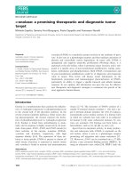
as illustrated in Figure 1. Even though a sequence

with n
H
= 6 yields a MAP estimate of
ˆ
θ = 0.6
(Figure 1 (a)), P (t = 1|w, θ) is only greater than
0.5 for a small range of θ around
ˆ
θ (Figure 1 (b)),
meaning that the choice of t = 1 is not very robust to
variation in θ. In contrast, a sequence with n
H
= 8
favors t = 1 for a wide range of θ around
ˆ
θ. By
integrating over θ, Equation 3 takes into account the
consequences of possible variation in θ.
Another advantage of integrating over θ is that
it permits the use of linguistically appropriate pri-
ors. In many linguistic models, including HMMs,
the distributions over variables are multinomial. For
a multinomial with parameters θ = (θ
1
, . , θ
K
), a
natural choice of prior is the K-dimensional Dirich-
let distribution, which is conjugate to the multino-
mial.

1
For simplicity, we initially assume that all
K parameters (also known as hyperparameters) of
the Dirichlet distribution are equal to β, i.e. the
Dirichlet is symmetric. The value of β determines
which parameters θ will have high probability: when
β = 1, all parameter values are equally likely; when
β > 1, multinomials that are closer to uniform are
1
A prior is conjugate to a distribution if the posterior has the
same form as the prior.
0 0.1 0.2 0.3 0.4 0.5 0.6 0.7 0.8 0.9 1
θ
P( θ | w )


0 0.1 0.2 0.3 0.4 0.5 0.6 0.7 0.8 0.9 1
0
0.5
1
θ
P( t = 1 | w, θ )


w = HHTHTTHHTH
w = HHTHHHTHHH
w = HHTHTTHHTH
w = HHTHHHTHHH
(a)
(b)

Figure 1: The Bayesian approach to estimating the
value of a latent variable, t, from observed data, w,
chooses a value of t robust to uncertainty in θ. (a)
Posterior distribution on θ given w. (b) Probability
that t = 1 given w and θ as a function of θ.
preferred; and when β < 1, high probability is as-
signed to sparse multinomials, where one or more
parameters are at or near 0.
Typically, linguistic structures are characterized
by sparse distributions (e.g., POS tags are followed
with high probability by only a few other tags, and
have highly skewed output distributions). Conse-
quently, it makes sense to use a Dirichlet prior with
β < 1. However, as noted by Johnson et al. (2007),
this choice of β leads to difficulties with MAP esti-
mation. For a sequence of draws x = (x
1
, . , x
n
)
from a multinomial distribution θ with observed
counts n
1
, . , n
K
, a symmetric Dirichlet(β) prior
over θ yields the MAP estimate θ
k
=
n

k
+β−1
n+K(β−1)
.
When β ≥ 1, standard MLE techniques such as
EM can be used to find the MAP estimate simply
by adding “pseudocounts” of size β − 1 to each of
the expected counts n
k
at each iteration. However,
when β < 1, the values of θ that set one or more
of the θ
k
equal to 0 can have infinitely high poste-
rior probability, meaning that MAP estimation can
yield degenerate solutions. If, instead of estimating
θ, we integrate over all possible values, we no longer
encounter such difficulties. Instead, the probability
that outcome x
i
takes value k given previous out-
comes x
−i
= (x
1
, . , x
i−1
) is
P (k|x
−i

, β) =

P (k|θ)P (θ|x
−i
, β) dθ
=
n
k
+ β
i − 1 + Kβ
(5)
746
where n
k
is the number of times k occurred in x
−i
.
See MacKay and Peto (1995) for a derivation.
2.2 Model Definition
Our model has the structure of a standard trigram
HMM, with the addition of symmetric Dirichlet pri-
ors over the transition and output distributions:
t
i
|t
i−1
= t, t
i−2
= t
′

, τ
(t,t
′
)
∼ Mult(τ
(t,t
′
)
)
w
i
|t
i
= t, ω
(t)
∼ Mult(ω
(t)
)
τ
(t,t
′
)
|α ∼ Dirichlet(α)
ω
(t)
|β ∼ Dirichlet(β)
where t
i
and w
i

are the ith tag and word. We assume
that sentence boundaries are marked with a distin-
guished tag. For a model with T possible tags, each
of the transition distributions τ
(t,t
′
)
has T compo-
nents, and each of the output distributions ω
(t)
has
W
t
components, where W
t
is the number of word
types that are permissible outputs for tag t. We will
use τ and ω to refer to the entire transition and out-
put parameter sets. This model assumes that the
prior over state transitions is the same for all his-
tories, and the prior over output distributions is the
same for all states. We relax the latter assumption in
Section 4.
Under this model, Equation 5 gives us
P (t
i
|t
−i
, α) =
n

(t
i−2
,t
i−1
,t
i
)
+ α
n
(t
i−2
,t
i−1
)
+ T α
(6)
P (w
i
|t
i
, t
−i
, w
−i
, β) =
n
(t
i
,w
i

)
+ β
n
(t
i
)
+ W
t
i
β
(7)
where n
(t
i−2
,t
i−1
,t
i
)
and n
(t
i
,w
i
)
are the number of
occurrences of the trigram (t
i−2
, t
i−1

, t
i
) and the
tag-word pair (t
i
, w
i
) in the i − 1 previously gener-
ated tags and words. Note that, by integrating out
the parameters τ and ω, we induce dependencies
between the variables in the model. The probabil-
ity of generating a particular trigram tag sequence
(likewise, output) depends on the number of times
that sequence (output) has been generated previ-
ously. Importantly, trigrams (and outputs) remain
exchangeable: the probability of a set of trigrams
(outputs) is the same regardless of the order in which
it was generated. The property of exchangeability is
crucial to the inference algorithm we describe next.
2.3 Inference
To perform inference in our model, we use Gibbs
sampling (Geman and Geman, 1984), a stochastic
procedure that produces samples from the posterior
distribution P (t|w, α, β) ∝ P (w|t, β)P (t|α). We
initialize the tags at random, then iteratively resam-
ple each tag according to its conditional distribution
given the current values of all other tags. Exchange-
ability allows us to treat the current counts of the
other tag trigrams and outputs as “previous” obser-
vations. The only complication is that resampling

a tag changes the identity of three trigrams at once,
and we must account for this in computing its condi-
tional distribution. The sampling distribution for t
i
is given in Figure 2.
In Bayesian statistical inference, multiple samples
from the posterior are often used in order to obtain
statistics such as the expected values of model vari-
ables. For POS tagging, estimates based on multi-
ple samples might be useful if we were interested in,
for example, the probability that two words have the
same tag. However, computing such probabilities
across all pairs of words does not necessarily lead to
a consistent clustering, and the result would be diffi-
cult to evaluate. Using a single sample makes stan-
dard evaluation methods possible, but yields sub-
optimal results because the value for each tag is sam-
pled from a distribution, and some tags will be as-
signed low-probability values. Our solution is to
treat the Gibbs sampler as a stochastic search pro-
cedure with the goal of identifying the MAP tag se-
quence. This can be done using tempering (anneal-
ing), where a temperature of φ is equivalent to rais-
ing the probabilities in the sampling distribution to
the power of
1
φ
. As φ approaches 0, even a single
sample will provide a good MAP estimate.
3 Fixed Hyperparameter Experiments

3.1 Method
Our initial experiments follow in the tradition begun
by Merialdo (1994), using a tag dictionary to con-
strain the possible parts of speech allowed for each
word. (This also fixes W
t
, the number of possible
words for tag t.) The dictionary was constructed by
listing, for each word, all tags found for that word in
the entire WSJ treebank. For the experiments in this
section, we used a 24,000-word subset of the tree-
747
P (t
i
|t
−i
, w, α, β) ∝
n
(t
i
,w
i
)
+ β
n
t
i
+ W
t
i

β
·
n
(t
i−2
,t
i−1
,t
i
)
+ α
n
(t
i−2
,t
i−1
)
+ T α
·
n
(t
i−1
,t
i
,t
i+1
)
+ I(t
i−2
= t

i−1
= t
i
= t
i+1
) + α
n
(t
i−1
,t
i
)
+ I(t
i−2
= t
i−1
= t
i
) + Tα
·
n
(t
i
,t
i+1
,t
i+2
)
+ I(t
i−2

= t
i
= t
i+2
, t
i−1
= t
i+1
) + I(t
i−1
= t
i
= t
i+1
= t
i+2
) + α
n
(t
i
,t
i+1
)
+ I(t
i−2
= t
i
, t
i−1
= t

i+1
) + I(t
i−1
= t
i
= t
i+1
) + T α
Figure 2: Conditional distribution for t
i
. Here, t
−i
refers to the current values of all tags except for t
i
, I(.)
is a function that takes on the value 1 when its argument is true and 0 otherwise, and all counts n
x
are with
respect to the tag trigrams and tag-word pairs in (t
−i
, w
−i
).
bank as our unlabeled training corpus. 54.5% of the
tokens in this corpus have at least two possible tags,
with the average number of tags per token being 2.3.
We varied the values of the hyperparameters α and
β and evaluated overall tagging accuracy. For com-
parison with our Bayesian HMM (BHMM) in this
and following sections, we also present results from

the Viterbi decoding of an HMM trained using MLE
by running EM to convergence (MLHMM). Where
direct comparison is possible, we list the scores re-
ported by Smith and Eisner (2005) for their condi-
tional random field model trained using contrastive
estimation (CRF/CE).
2
For all experiments, we ran our Gibbs sampling
algorithm for 20,000 iterations over the entire data
set. The algorithm was initialized with a random tag
assignment and a temperature of 2, and the temper-
ature was gradually decreased to .08. Since our in-
ference procedure is stochastic, our reported results
are an average over 5 independent runs.
Results from our model for a range of hyperpa-
rameters are presented in Table 1. With the best
choice of hyperparameters (α = .003, β = 1), we
achieve average tagging accuracy of 86.8%. This
far surpasses the MLHMM performance of 74.5%,
and is closer to the 90.1% accuracy of CRF/CE on
the same data set using oracle parameter selection.
The effects of α, which determines the probabil-
2
Results of CRF/CE depend on the set of features used and
the contrast neighborhood. In all cases, we list the best score
reported for any contrast neighborhood using trigram (but no
spelling) features. To ensure proper comparison, all corpora
used in our experiments consist of the same randomized sets of
sentences used by Smith and Eisner. Note that training on sets
of contiguous sentences from the beginning of the treebank con-

sistently improves our results, often by 1-2 percentage points or
more. MLHMM scores show less difference between random-
ized and contiguous corpora.
Value
Value of β
of α
.001 .003 .01 .03 .1 .3 1.0
.001 85.0 85.7 86.1 86.0 86.2 86.5 86.6
.003
85.5 85.5 85.8 86.6 86.7 86.7 86.8
.01
85.3 85.5 85.6 85.9 86.4 86.4 86.2
.03
85.9 85.8 86.1 86.2 86.6 86.8 86.4
.1
85.2 85.0 85.2 85.1 84.9 85.5 84.9
.3
84.4 84.4 84.6 84.4 84.5 85.7 85.3
1.0
83.1 83.0 83.2 83.3 83.5 83.7 83.9
Table 1: Percentage of words tagged correctly by
BHMM as a function of the hyperparameters α and
β. Results are averaged over 5 runs on the 24k cor-
pus with full tag dictionary. Standard deviations in
most cases are less than .5.
ity of the transition distributions, are stronger than
the effects of β, which determines the probability
of the output distributions. The optimal value of
.003 for α reflects the fact that the true transition
probability matrix for this corpus is indeed sparse.

As α grows larger, the model prefers more uniform
transition probabilities, which causes it to perform
worse. Although the true output distributions tend to
be sparse as well, the level of sparseness depends on
the tag (consider function words vs. content words
in particular). Therefore, a value of β that accu-
rately reflects the most probable output distributions
for some tags may be a poor choice for other tags.
This leads to the smaller effect of β, and suggests
that performance might be improved by selecting a
different β for each tag, as we do in the next section.
A final point worth noting is that even when
α = β = 1 (i.e., the Dirichlet priors exert no influ-
ence) the BHMM still performs much better than the
MLHMM. This result underscores the importance
of integrating over model parameters: the BHMM
identifies a sequence of tags that have high proba-
748
bility over a range of parameter values, rather than
choosing tags based on the single best set of para-
meters. The improved results of the BHMM demon-
strate that selecting a sequence that is robust to vari-
ations in the parameters leads to better performance.
4 Hyperparameter Inference
In our initial experiments, we experimented with dif-
ferent fixed values of the hyperparameters and re-
ported results based on their optimal values. How-
ever, choosing hyperparameters in this way is time-
consuming at best and impossible at worst, if there
is no gold standard available. Luckily, the Bayesian

approach allows us to automatically select values
for the hyperparameters by treating them as addi-
tional variables in the model. We augment the model
with priors over the hyperparameters (here, we as-
sume an improper uniform prior), and use a sin-
gle Metropolis-Hastings update (Gilks et al., 1996)
to resample the value of each hyperparameter after
each iteration of the Gibbs sampler. Informally, to
update the value of hyperparameter α, we sample a
proposed new value α
′
from a normal distribution
with µ = α and σ = .1α. The probability of ac-
cepting the new value depends on the ratio between
P (t|w, α) and P (t|w, α
′
) and a term correcting for
the asymmetric proposal distribution.
Performing inference on the hyperparameters al-
lows us to relax the assumption that every tag has
the same prior on its output distribution. In the ex-
periments reported in the following section, we used
two different versions of our model. The first ver-
sion (BHMM1) uses a single value of β for all word
classes (as above); the second version (BHMM2)
uses a separate β
j
for each tag class j.
5 Inferred Hyperparameter Experiments
5.1 Varying corpus size

In this set of experiments, we used the full tag dictio-
nary (as above), but performed inference on the hy-
perparameters. Following Smith and Eisner (2005),
we trained on four different corpora, consisting of
the first 12k, 24k, 48k, and 96k words of the WSJ
corpus. For all corpora, the percentage of ambigu-
ous tokens is 54%-55% and the average number of
tags per token is 2.3. Table 2 shows results for
the various models and a random baseline (averaged
Corpus size
Accuracy
12k 24k 48k 96k
random 64.8 64.6 64.6 64.6
MLHMM
71.3 74.5 76.7 78.3
CRF/CE
86.2 88.6 88.4 89.4
BHMM1
85.8 85.2 83.6 85.0
BHMM2
85.8 84.4 85.7 85.8
σ <
.7 .2 .6 .2
Table 2: Percentage of words tagged correctly
by the various models on different sized corpora.
BHMM1 and BHMM2 use hyperparameter infer-
ence; CRF/CE uses parameter selection based on an
unlabeled development set. Standard deviations (σ)
for the BHMM results fell below those shown for
each corpus size.

over 5 random tag assignments). Hyperparameter
inference leads to slightly lower scores than are ob-
tained by oracle hyperparameter selection, but both
versions of BHMM are still far superior to MLHMM
for all corpus sizes. Not surprisingly, the advantages
of BHMM are most pronounced on the smallest cor-
pus: the effects of parameter integration and sensible
priors are stronger when less evidence is available
from the input. In the limit as corpus size goes to in-
finity, the BHMM and MLHMM will make identical
predictions.
5.2 Varying dictionary knowledge
In unsupervised learning, it is not always reasonable
to assume that a large tag dictionary is available. To
determine the effects of reduced or absent dictionary
information, we ran a set of experiments inspired
by those of Smith and Eisner (2005). First, we col-
lapsed the set of 45 treebank tags onto a smaller set
of 17 (the same set used by Smith and Eisner). We
created a full tag dictionary for this set of tags from
the entire treebank, and also created several reduced
dictionaries. Each reduced dictionary contains the
tag information only for words that appear at least
d times in the training corpus (the 24k corpus, for
these experiments). All other words are fully am-
biguous between all 17 classes. We ran tests with
d = 1, 2, 3, 5, 10, and ∞ (i.e., knowledge-free syn-
tactic clustering).
With standard accuracy measures, it is difficult to
749

Value of d
Accuracy
1 2 3 5 10 ∞
random 69.6 56.7 51.0 45.2 38.6
MLHMM
83.2 70.6 65.5 59.0 50.9
CRF/CE
90.4 77.0 71.7
BHMM1
86.0 76.4 71.0 64.3 58.0
BHMM2
87.3 79.6 65.0 59.2 49.7
σ <
.2 .8 .6 .3 1.4
VI
random 2.65 3.96 4.38 4.75 5.13 7.29
MLHMM
1.13 2.51 3.00 3.41 3.89 6.50
BHMM1
1.09 2.44 2.82 3.19 3.47 4.30
BHMM2
1.04 1.78 2.31 2.49 2.97 4.04
σ <
.02 .03 .04 .03 .07 .17
Corpus stats
% ambig. 49.0 61.3 66.3 70.9 75.8 100
tags/token
1.9 4.4 5.5 6.8 8.3 17
Table 3: Percentage of words tagged correctly and
variation of information between clusterings in-

duced by the assigned and gold standard tags as the
amount of information in the dictionary is varied.
Standard deviations (σ ) for the BHMM results fell
below those shown in each column. The percentage
of ambiguous tokens and average number of tags per
token for each value of d is also shown.
evaluate the quality of a syntactic clustering when
no dictionary is used, since cluster names are inter-
changeable. We therefore introduce another evalua-
tion measure for these experiments, a distance met-
ric on clusterings known as variation of information
(Meilˇa, 2002). The variation of information (VI) be-
tween two clusterings C (the gold standard) and C
′
(the found clustering) of a set of data points is a sum
of the amount of information lost in moving from C
to C
′
, and the amount that must be gained. It is de-
fined in terms of entropy H and mutual information
I: V I(C, C
′
) = H(C) + H(C
′
) − 2I(C, C
′
). Even
when accuracy can be measured, VI may be more in-
formative: two different tag assignments may have
the same accuracy but different VI with respect to

the gold standard if the errors in one assignment are
less consistent than those in the other.
Table 3 gives the results for this set of experi-
ments. One or both versions of BHMM outperform
MLHMM in terms of tag accuracy for all values of
d, although the differences are not as great as in ear-
lier experiments. The differences in VI are more
striking, particularly as the amount of dictionary in-
formation is reduced. When ambiguity is greater,
both versions of BHMM show less confusion with
respect to the true tags than does MLHMM, and
BHMM2 performs the best in all circumstances. The
confusion matrices in Figure 3 provide a more intu-
itive picture of the very different sorts of clusterings
produced by MLHMM and BHMM2 when no tag
dictionary is available. Similar differences hold to a
lesser degree when a partial dictionary is provided.
With MLHMM, different tokens of the same word
type are usually assigned to the same cluster, but
types are assigned to clusters more or less at ran-
dom, and all clusters have approximately the same
number of types (542 on average, with a standard
deviation of 174). The clusters found by BHMM2
tend to be more coherent and more variable in size:
in the 5 runs of BHMM2, the average number of
types per cluster ranged from 436 to 465 (i.e., to-
kens of the same word are spread over fewer clus-
ters than in MLHMM), with a standard deviation
between 460 and 674. Determiners, prepositions,
the possessive marker, and various kinds of punc-

tuation are mostly clustered coherently. Nouns are
spread over a few clusters, partly due to a distinction
found between common and proper nouns. Like-
wise, modal verbs and the copula are mostly sep-
arated from other verbs. Errors are often sensible:
adjectives and nouns are frequently confused, as are
verbs and adverbs.
The kinds of results produced by BHMM1 and
BHMM2 are more similar to each other than to
the results of MLHMM, but the differences are still
informative. Recall that BHMM1 learns a single
value for β that is used for all output distribu-
tions, while BHMM2 learns separate hyperparame-
ters for each cluster. This leads to different treat-
ments of difficult-to-classify low-frequency items.
In BHMM1, these items tend to be spread evenly
among all clusters, so that all clusters have simi-
larly sparse output distributions. In BHMM2, the
system creates one or two clusters consisting en-
tirely of very infrequent items, where the priors on
these clusters strongly prefer uniform outputs, and
all other clusters prefer extremely sparse outputs
(and are more coherent than in BHMM1). This
explains the difference in VI between the two sys-
tems, as well as the higher accuracy of BHMM1
for d ≥ 3: the single β discourages placing low-
frequency items in their own cluster, so they are
more likely to be clustered with items that have sim-
750
1 2 3 4 5 6 7 8 9 1011121314151617

N
INPUNC
ADJ
V
DET
PREP
ENDPUNC
VBG
CONJ
VBN
ADV
TO
WH
PRT
POS
LPUNC
RPUNC
(a) BHMM2
Found Tags
True Tags
1 2 3 4 5 6 7 8 9 1011121314151617
N
INPUNC
ADJ
V
DET
PREP
ENDPUNC
VBG
CONJ

VBN
ADV
TO
WH
PRT
POS
LPUNC
RPUNC
(b) MLHMM
Found Tags
True Tags
Figure 3: Confusion matrices for the dictionary-free clusterings found by (a) BHMM2 and (b) MLHMM.
ilar transition probabilities. The problem of junk
clusters in BHMM2 might be alleviated by using a
non-uniform prior over the hyperparameters to en-
courage some degree of sparsity in all clusters.
6 Conclusion
In this paper, we have demonstrated that, for a stan-
dard trigram HMM, taking a Bayesian approach
to POS tagging dramatically improves performance
over maximum-likelihood estimation. Integrating
over possible parameter values leads to more robust
solutions and allows the use of priors favoring sparse
distributions. The Bayesian approach is particularly
helpful when learning is less constrained, either be-
cause less data is available or because dictionary
information is limited or absent. For knowledge-
free clustering, our approach can also be extended
through the use of infinite models so that the num-
ber of clusters need not be specified in advance. We

hope that our success with POS tagging will inspire
further research into Bayesian methods for other nat-
ural language learning tasks.
References
M. Banko and R. Moore. 2004. A study of unsupervised part-
of-speech tagging. In Proceedings of COLING ’04.
E. Brill. 1995. Unsupervised learning of disambiguation rules
for part of speech tagging. In Proceedings of the 3rd Work-
shop on Very Large Corpora, pages 1–13.
P. Brown, V. Della Pietra, V. de Souza, J. Lai, and R. Mer-
cer. 1992. Class-based n-gram models of natural language.
Computational Linguistics, 18:467–479.
A. Clark. 2000. Inducing syntactic categories by context dis-
tribution clustering. In Proceedings of the Conference on
Natural Language Learning (CONLL).
S. Finch, N. Chater, and M. Redington. 1995. Acquiring syn-
tactic information from distributional statistics. In J. In Levy,
D. Bairaktaris, J. Bullinaria, and P. Cairns, editors, Connec-
tionist Models of Memory and Language. UCL Press, Lon-
don.
S. Geman and D. Geman. 1984. Stochastic relaxation, Gibbs
distributions and the Bayesian restoration of images. IEEE
Transactions on Pattern Analysis and Machine Intelligence,
6:721–741.
W.R. Gilks, S. Richardson, and D. J. Spiegelhalter, editors.
1996. Markov Chain Monte Carlo in Practice. Chapman
and Hall, Suffolk.
A. Haghighi and D. Klein. 2006. Prototype-driven learning for
sequence models. In Proceedings of HLT-NAACL.
M. Johnson, T. Griffiths, and S. Goldwater. 2007. Bayesian

inference for PCFGs via Markov chain Monte Carlo.
D. Klein and C. Manning. 2002. A generative constituent-
context model for improved grammar induction. In Proceed-
ings of the ACL.
D. MacKay and L. Bauman Peto. 1995. A hierarchical Dirich-
let language model. Natural Language Engineering, 1:289–
307.
M. Meilˇa. 2002. Comparing clusterings. Technical Report 418,
University of Washington Statistics Department.
B. Merialdo. 1994. Tagging English text with a probabilistic
model. Computational Linguistics, 20(2):155–172.
L. Saul and F. Pereira. 1997. Aggregate and mixed-order
markov models for statistical language processing. In Pro-
ceedings of the Second Conference on Empirical Methods in
Natural Language Processing (EMNLP).
H. Sch¨utze. 1995. Distributional part-of-speech tagging. In
Proceedings of the European Chapter of the Association for
Computational Linguistics (EACL).
N. Smith and J. Eisner. 2005. Contrastive estimation: Training
log-linear models on unlabeled data. In Proceedings of ACL.
I. Wang and D. Schuurmans. 2005. Improved estimation
for unsupervised part-of-speech tagging. In Proceedings
of the IEEE International Conference on Natural Language
Processing and Knowledge Engineering (IEEE NLP-KE).
751