Báo cáo khoa học: "Redundancy Ratio: An Invariant Property of the Consonant Inventories of the World’s Languages" pdf
Bạn đang xem bản rút gọn của tài liệu. Xem và tải ngay bản đầy đủ của tài liệu tại đây (366.72 KB, 8 trang )
Proceedings of the 45th Annual Meeting of the Association of Computational Linguistics, pages 104–111,
Prague, Czech Republic, June 2007.
c
2007 Association for Computational Linguistics
Redundancy Ratio: An Invariant Property of the
Consonant Inventories of the World’s Languages
Animesh Mukherjee, Monojit Choudhury, Anupam Basu, Niloy Ganguly
Department of Computer Science and Engineering,
Indian Institute of Technology, Kharagpur
{animeshm,monojit,anupam,niloy}@cse.iitkgp.ernet.in
Abstract
In this paper, we put forward an information
theoretic definition of the redundancy that is
observed across the sound inventories of the
world’s languages. Through rigorous statis-
tical analysis, we find that this redundancy
is an invariant property of the consonant in-
ventories. The statistical analysis further un-
folds that the vowel inventories do not ex-
hibit any such property, which in turn points
to the fact that the organizing principles of
the vowel and the consonant inventories are
quite different in nature.
1 Introduction
Redundancy is a strikingly common phenomenon
that is observed across many natural systems. This
redundancy is present mainly to reduce the risk
of the complete loss of information that might oc-
cur due to accidental errors (Krakauer and Plotkin,
2002). Moreover, redundancy is found in every level
of granularity of a system. For instance, in biologi-
cal systems we find redundancy in the codons (Lesk,
2002), in the genes (Woollard, 2005) and as well in
the proteins (Gatlin, 1974). A linguistic system is
also not an exception. There is for example, a num-
ber of words with the same meaning (synonyms) in
almost every language of the world. Similarly, the
basic unit of language, the human speech sounds or
the phonemes, is also expected to exhibit some sort
of a redundancy in the information that it encodes.
In this work, we attempt to mathematically cap-
ture the redundancy observed across the sound
(more specifically the consonant) inventories of
the world’s languages. For this purpose, we
present an information theoretic definition of redun-
dancy, which is calculated based on the set of fea-
tures
1
(Trubetzkoy, 1931) that are used to express
the consonants. An interesting observation is that
this quantitative feature-based measure of redun-
dancy is almost an invariance over the consonant
inventories of the world’s languages. The observa-
tion is important since it can shed enough light on
the organization of the consonant inventories, which
unlike the vowel inventories, lack a complete and
holistic explanation. The invariance of our measure
implies that every inventory tries to be similar in
terms of the measure, which leads us to argue that
redundancy plays a very important role in shaping
the structure of the consonant inventories. In order
to validate this argument we determine the possibil-
ity of observing such an invariance if the consonant
inventories had evolved by random chance. We find
that the redundancy observed across the randomly
generated inventories is substantially different from
their real counterparts, which leads us to conclude
that the invariance is not just “by-chance” and the
measure that we define, indeed, largely governs the
organizing principles of the consonant inventories.
1
In phonology, features are the elements, which distin-
guish one phoneme from another. The features that distinguish
the consonants can be broadly categorized into three different
classes namely the manner of articulation, the place of articu-
lation and phonation. Manner of articulation specifies how the
flow of air takes place in the vocal tract during articulation of
a consonant, whereas place of articulation specifies the active
speech organ and also the place where it acts. Phonation de-
scribes the activity regarding the vibration of the vocal cords
during the articulation of a consonant.
104
Interestingly, this redundancy, when measured for
the vowel inventories, does not exhibit any similar
invariance. This immediately reveals that the prin-
ciples that govern the formation of these two types
of inventories are quite different in nature. Such
an observation is significant since whether or not
these principles are similar/different for the two in-
ventories had been a question giving rise to peren-
nial debate among the past researchers (Trubet-
zkoy, 1969/1939; Lindblom and Maddieson, 1988;
Boersma, 1998; Clements, 2004). A possible rea-
son for the observed dichotomy in the behavior of
the vowel and consonant inventories with respect to
redundancy can be as follows: while the organiza-
tion of the vowel inventories is known to be gov-
erned by a single force - the maximal perceptual
contrast (Jakobson, 1941; Liljencrants and Lind-
blom, 1972; de Boer, 2000)), consonant invento-
ries are shaped by a complex interplay of several
forces (Mukherjee et al., 2006). The invariance of
redundancy, perhaps, reflects some sort of an equi-
librium that arises from the interaction of these di-
vergent forces.
The rest of the paper is structured as follows. In
section 2 we briefly discuss the earlier works in con-
nection to the sound inventories and then systemat-
ically build up the quantitative definition of redun-
dancy from the linguistic theories that are already
available in the literature. Section 3 details out the
data source necessary for the experiments, describes
the baseline for the experiments, reports the exper-
iments performed, and presents the results obtained
each time comparing the same with the baseline re-
sults. Finally we conclude in section 4 by summa-
rizing our contributions, pointing out some of the
implications of the current work and indicating the
possible future directions.
2 Formulation of Redundancy
Linguistic research has documented a wide range of
regularities across the sound systems of the world’s
languages. It has been postulated earlier by func-
tional phonologists that such regularities are thecon-
sequences of certain general principles like maxi-
mal perceptual contrast (Liljencrants and Lindblom,
1972), which is desirable between the phonemes of
a language for proper perception of each individ-
ual phoneme in a noisy environment, ease of artic-
ulation (Lindblom and Maddieson, 1988; de Boer,
2000), which requires that the sound systems of
all languages are formed of certain universal (and
highly frequent) sounds, and ease of learnability (de
Boer, 2000), which is necessary for a speaker to
learn the sounds of a language with minimum ef-
fort. In fact, the organization of the vowel inven-
tories (especially those with a smaller size) across
languages has been satisfactorily explained in terms
of the single principle of maximal perceptual con-
trast (Jakobson, 1941; Liljencrants and Lindblom,
1972; de Boer, 2000).
On the other hand, in spite of several at-
tempts (Lindblom and Maddieson, 1988; Boersma,
1998; Clements, 2004) the organization of the con-
sonant inventories lacks a satisfactory explanation.
However, one of the earliest observations about the
consonant inventories has been that consonants tend
to occur in pairs that exhibit strong correlation in
terms of their features (Trubetzkoy, 1931). In or-
der to explain these trends, feature economy was
proposed as the organizing principle of the con-
sonant inventories (Martinet, 1955). According to
this principle, languages tend to maximize the com-
binatorial possibilities of a few distinctive features
to generate a large number of consonants. Stated
differently, a given consonant will have a higher
than expected chance of occurrence in inventories in
which all of its features have distinctively occurred
in other consonants. The idea is illustrated, with an
example, through Table 1. Various attempts have
been made in the past to explain the aforementioned
trends through linguistic insights (Boersma, 1998;
Clements, 2004) mainly establishing their statistical
significance. On the contrary, there has been very
little work pertaining to the quantification of feature
economy except in (Clements, 2004), where the au-
thor defines economy index, which is the ratio of the
size of an inventory to the number of features that
characterizes the inventory. However, this definition
does not take into account the complexity that is in-
volved in communicating the information about the
inventory in terms of its constituent features.
Inspired by the aforementioned studies and
the concepts of information theory (Shannon and
Weaver, 1949) we try to quantitatively capture the
amount of redundancy found across the consonant
105
plosive voiced voiceless
dental /d/ /t/
bilabial /b/ /p/
Table 1: The table shows four plosives. If a language
has in its consonant inventory any three of the four
phonemes listed in this table, then there is a higher
than average chance that it will also have the fourth
phoneme of the table in its inventory.
inventories in terms of their constituent features. Let
us assume that we want to communicate the infor-
mation about an inventory of size N over a transmis-
sion channel. Ideally, one should require log N bits
to do the same (where the logarithm is with respect
to base 2). However, since every natural system is
to some extent redundant and languages are no ex-
ceptions, the number of bits actually used to encode
the information is more than log N. If we assume
that the features are boolean in nature, then we can
compute the number of bits used by a language to
encode the information about its inventory by mea-
suring the entropy as follows. For an inventory of
size N let there be p
f
consonants for which a partic-
ular feature f (where f is assumed to be boolean in
nature) is present and q
f
other consonants for which
the same is absent. Thus the probability that a par-
ticular consonant chosen uniformly at random from
this inventory has the feature f is
p
f
N
and the prob-
ability that the consonant lacks the feature f is
q
f
N
(=1–
p
f
N
). If F is the set of all features present in
the consonants forming the inventory, then feature
entropy F
E
can be expressed as
F
E
=
f∈F
(−
p
f
N
log
p
f
N
−
q
f
N
log
q
f
N
) (1)
F
E
is therefore the measure of the minimum number
of bits that is required to communicate the informa-
tion about the entire inventory through the transmis-
sion channel. The lower the value of F
E
the better
it is in terms of the information transmission over-
head. In order to capture the redundancy involved in
the encoding we define the term redundancy ratio as
follows,
RR =
F
E
log N
(2)
which expresses the excess number of bits that is
used by the constituent consonants of the inventory
Figure 1: The process of computing RR for a hypo-
thetical inventory.
in terms of a ratio. The process of computing the
value of RR for a hypothetical consonant inventory
is illustrated in Figure 1.
In the following section, we present the experi-
mental setup and also report the experiments which
we perform based on the above definition of redun-
dancy. We subsequently show that redundancy ratio
is invariant across the consonant inventories whereas
the same is not true in the case of the vowel invento-
ries.
3 Experiments and Results
In this section we discuss the data source necessary
for the experiments, describe the baseline for the
experiments, report the experiments performed, and
present the results obtained each time comparing the
same with the baseline results.
3.1 Data Source
Many typological studies (Ladefoged and Mad-
dieson, 1996; Lindblom and Maddieson, 1988)
of segmental inventories have been carried out in
past on the UCLA Phonological Segment Inven-
tory Database (UPSID) (Maddieson, 1984). UPSID
gathers phonological systems of languages from all
over the world, sampling more or less uniformly all
the linguistic families. In this work we have used
UPSID comprising of 317 languages and 541 con-
sonants found across them, for our experiments.
106
3.2 Redundancy Ratio across the Consonant
Inventories
In this section we measure the redundancy ratio (de-
scribed earlier) of the consonant inventories of the
languages recorded in UPSID. Figure 2 shows the
scatter-plot of the redundancy ratio R R of each of
the consonant inventories (y-axis) versus the inven-
tory size (x-axis). The plot immediately reveals that
the measure (i.e., RR ) is almost invariant across the
consonant inventories with respect to the inventory
size. In fact, we can fit the scatter-plot with a straight
line (by means of least square regression), which as
depicted in Figure 2, has a negligible slope (m = –
0.018) and this in turn further confirms the above
fact that RR is an invariant property of the conso-
nant inventories with regard to their size. It is im-
portant to mention here that in this experiment we
report the redundancy ratio of all the inventories of
size less than or equal to 40. We neglect the inven-
tories of the size greater than 40 since they are ex-
tremely rare (less than 0.5% of the languages of UP-
SID), and therefore, cannot provide us with statis-
tically meaningful estimates. The same convention
has been followed in all the subsequent experiments.
Nevertheless, we have also computed the values of
RR for larger inventories, whereby we have found
that for an inventory size ≤ 60 the results are sim-
ilar to those reported here. It is interesting to note
that the largest of the consonant inventories Ga (size
= 173) has an RR = 1.9, which is lower than all the
other inventories.
The aforementioned claim that RR is an invari-
ant across consonant inventories can be validated by
performing a standard test of hypothesis. For this
purpose, we randomly construct language invento-
ries, as discussed later, and formulate a null hypoth-
esis based on them.
Null Hypothesis: The invariance in the distribution
of RRs observed across the real consonant invento-
ries is also prevalent across the randomly generated
inventories.
Having formulated the null hypothesis we now
systematically attempt to reject the same with a very
high probability. For this purpose we first construct
random inventories and then perform a two sample
t-test (Cohen, 1995) comparing the RRs of the real
and the random inventories. The results show that
Figure 2: The scatter-plot of the redundancy ratio
RR of each of the consonant inventories (y-axis)
versus the inventory size (x-axis). The straight line-
fit is also depicted by the bold line in the figure.
indeed the null hypothesis can be rejected with a
very high probability. We proceed as follows.
3.2.1 Construction of Random Inventories
We employ two different models to generate the
random inventories. In the first model the invento-
ries are filled uniformly at random from the pool of
541 consonants. In the second model we assume
that the distribution of the occurrence of the conso-
nants over languages is known a priori. Note that
in both of these cases, the size of the random in-
ventories is same as its real counterpart. The results
show that the distribution of RR s obtained from the
second model has a closer match with the real in-
ventories than that of the first model. This indicates
that the occurrence frequency to some extent gov-
erns the law of organization of the consonant inven-
tories. The detail of each of the models follow.
Model I – Purely Random Model: In this model
we assume that the distribution of the consonant in-
ventory size is known a priori. For each language
inventory L let the size recorded in UPSID be de-
noted by s
L
. Let there be 317 bins corresponding to
each consonant inventory L. A bin corresponding to
an inventory L is packed with s
L
consonants chosen
uniformly at random (without repetition) from the
pool of 541 available consonants. Thus the conso-
nant inventories of the 317 languages corresponding
to the bins are generated. The method is summarized
107
in Algorithm 1.
for I = 1 to 317 do
for size = 1 to s
L
do
Choose a consonant c uniformly at
random (without repetition) from the
pool of 541 available consonants;
Pack the consonant c in the bin
corresponding to the inventory L;
end
end
Algorithm 1: Algorithm to construct random in-
ventories using Model I
Model II – Occurrence Frequency based Random
Model: For each consonant c let the frequency of
occurrence in UPSID be denoted by f
c
. Let there be
317 bins each corresponding to a language in UP-
SID. f
c
bins are then chosen uniformly at random
and the consonant c is packed into these bins. Thus
the consonant inventories of the 317 languages cor-
responding to the bins are generated. The entire idea
is summarized in Algorithm 2.
for each consonant c do
for i = 1 to f
c
do
Choose one of the 317 bins,
corresponding to the languages in
UPSID, uniformly at random;
Pack the consonant c into the bin so
chosen if it has not been already packed
into this bin earlier;
end
end
Algorithm 2: Algorithm to construct random in-
ventories using Model II
3.2.2 Results Obtained from the Random
Models
In this section we enumerate the results obtained
by computing the RRs of the randomly generated
inventories using Model I and Model II respectively.
We compare the results with those of the real inven-
Parameters Real Inv. Random Inv.
Mean 2.51177 3.59331
SDV 0.209531 0.475072
Parameters Values
t 12.15
DF 66
p ≤ 9.289e-17
Table 2: The results of the t-test comparing the dis-
tribution of RRs for the real and the random invento-
ries (obtained through Model I). SDV: standard devi-
ation, t: t-value of the test, DF: degrees of freedom,
p: residual uncertainty.
tories and in each case show that the null hypothesis
can be rejected with a significantly high probability.
Results from Model I: Figure 3 illustrates, for all
the inventories obtained from 100 different simula-
tion runs of Algorithm 1, the average redundancy
ratio exhibited by the inventories of a particular size
(y-axis), versus the inventory size (x-axis). The
term “redundancy ratio exhibited by the inventories
of a particular size” actually means the following.
Let there be n consonant inventories of a particu-
lar inventory-size k. The average redundancy ra-
tio of the inventories of size k is therefore given by
1
n
n
i=1
RR
i
where RR
i
signifies the redundancy ra-
tio of the i
th
inventory of size k. In Figure 3 we also
present the same curve for the real consonant inven-
tories appearing in UPSID. In these curves we fur-
ther depict the error bars spanning the entire range of
values starting from the minimum RR to the max-
imum RR for a given inventory size. The curves
show that in case of real inventories the error bars
span a very small range as compared to that of the
randomly constructed ones. Moreover, the slopes of
the curves are also significantly different. In order
to test whether this difference is significant, we per-
form a t-test comparing the distribution of the val-
ues of RR that gives rise to such curves for the real
and the random inventories. The results of the test
are noted in Table 2. These statistics clearly shows
that the distribution of RRs for the real and the ran-
dom inventories are significantly different in nature.
Stated differently, we can reject the null hypothesis
with (100 - 9.29e-15)% confidence.
Results from Model II: Figure 4 illustrates, for
all the inventories obtained from 100 different simu-
108
Figure 3: Curves showing the average redundancy
ratio exhibited by the real as well as the random in-
ventories (obtained through Model I) of a particular
size (y-axis), versus the inventory size (x-axis).
lation runs of Algorithm 2, the average redundancy
ratio exhibited by the inventories of a particular size
(y-axis), versus the inventory size (x-axis). The fig-
ure shows the same curve for the real consonant in-
ventories also. For each of the curve, the error bars
span the entire range of values starting from the min-
imum RR to the maximum RR for a given inventory
size. It is quite evident from the figure that the error
bars for the curve representing the real inventories
are smaller than those of the random ones. The na-
ture of the two curves are also different though the
difference is not as pronounced as in case of Model I.
This is indicative of the fact that it is not only the oc-
currence frequency that governs the organization of
the consonant inventories and there is a more com-
plex phenomenon that results in such an invariant
property. In fact, in this case also, the t-test statistics
comparing the distribution of RRs for the real and
the random inventories, reported in Table 3, allows
us to reject the null hypothesis with (100–2.55e–3)%
confidence.
3.3 Comparison with Vowel Inventories
Until now we have been looking into the organiza-
tional aspects of the consonant inventories. In this
section we show that this organization is largely dif-
ferent from that of the vowel inventories in the sense
that there is no such invariance observed across the
vowel inventories unlike that of consonants. For
this reason we start by computing the RRs of all
Figure 4: Curves showing the average redundancy
ratio exhibited by the real as well as the random in-
ventories (obtained through Model II) of a particular
size (y-axis), versus the inventory size (x-axis).
Parameters Real Inv. Random Inv.
Mean 2.51177 2.76679
SDV 0.209531 0.228017
Parameters Values
t 4.583
DF 60
p ≤ 2.552e-05
Table 3: The results of the t-test comparing the dis-
tribution of RRs for the real and the random inven-
tories (obtained through Model II).
the vowel inventories appearing in UPSID. Figure 5
shows the scatter plot of the redundancy ratio of each
of the vowel inventories (y-axis) versus the inven-
tory size (x-axis). The plot clearly indicates that the
measure (i.e., R R) is not invariant across the vowel
inventories and in fact, the straight line that fits the
distribution has a slope of –0.14, which is around 10
times higher than that of the consonant inventories.
Figure 6 illustrates the average redundancy ratio
exhibited by the vowel and the consonant inventories
of a particular size (y-axis), versus the inventory size
(x-axis). The error bars indicating the variability of
RR among the inventories of a fixed size also span a
much larger range for the vowel inventories than for
the consonant inventories.
The significance of the difference in the nature of
the distribution of RRs for the vowel and the conso-
nant inventories can be again estimated by perform-
ing a t-test. The null hypothesis in this case is as
follows.
109
Figure 5: The scatter-plot of the redundancy ratio
RR of each of the vowel inventories (y-axis) versus
the inventory size (x-axis). The straight line-fit is
depicted by the bold line in the figure.
Figure 6: Curves showing the average redundancy
ratio exhibited by the vowel as well as the consonant
inventories of a particular size (y-axis), versus the
inventory size (x-axis).
Null Hypothesis: The nature of the distribution of
RRs for the vowel and the consonant inventories is
same.
We can now perform the t-test to verify whether
we can reject the above hypothesis. Table 4 presents
the results of the test. The statistics immediately
confirms that the null hypothesis can be rejected
with 99.932% confidence.
Parameters Consonant Inv. Vowel Inv.
Mean 2.51177 2.98797
SDV 0.209531 0.726547
Parameters Values
t 3.612
DF 54
p ≤ 0.000683
Table 4: The results of the t-test comparing the dis-
tribution of RRs for the consonant and the vowel
inventories.
4 Conclusions, Discussion and Future
Work
In this paper we have mathematically captured the
redundancy observed across the sound inventories of
the world’s languages. We started by systematically
defining the term redundancy ratio and measuring
the value of the same for the inventories. Some of
our important findings are,
1. Redundancy ratio is an invariant property of the
consonant inventories with respect to the inventory
size.
2. A more complex phenomenon than merely the
occurrence frequency results in such an invariance.
3. Unlike the consonant inventories, the vowel in-
ventories are not indicative of such an invariance.
Until now we have concentrated on establishing
the invariance of the redundancy ratio across the
consonant inventories rather than reasoning why it
could have emerged. One possible way to answer
this question is to look for the error correcting ca-
pability of the encoding scheme that nature had em-
ployed for characterization of the consonants. Ide-
ally, if redundancy has to be invariant, then this ca-
pability should be almost constant. As a proof of
concept we randomly select a consonant from in-
ventories of different size and compute its hamming
distance from the rest of the consonants in the inven-
tory. Figure 7 shows for a randomly chosen conso-
nant c from an inventory of size 10, 15, 20 and 30
respectively, the number of the consonants at a par-
ticular hamming distance from c (y-axis) versus the
hamming distance (x-axis). The curve clearly indi-
cates that majority of the consonants are at a ham-
ming distance of 4 from c, which in turn implies that
the encoding scheme has almost a fixed error cor-
recting capability of 1 bit. This can be the precise
reason behind the invariance of the redundancy ra-
110
Figure 7: Histograms showing the the number of consonants at a particular hamming distance (y-axis), from
a randomly chosen consonant c, versus the hamming distance (x-axis).
tio. Initial studies into the vowel inventories show
that for a randomly chosen vowel, its hamming dis-
tance from the other vowels in the same inventory
varies with the inventory size. In other words, the er-
ror correcting capability of a vowel inventory seems
to be dependent on the size of the inventory.
We believe that these results are significant as well
as insightful. Nevertheless, one should be aware of
the fact that the formulation of RR heavily banks
on the set of features that are used to represent the
phonemes. Unfortunately, there is no consensus on
the set of representative features, even though there
are numerous suggestions available in the literature.
However, the basic concept of RR and the process of
analysis presented here is independent of the choice
of the feature set. In the current study we have used
the binary features provided in UPSID, which could
be very well replaced by other representations, in-
cluding multi-valued feature systems; we look for-
ward to do the same as a part of our future work.
References
B. de Boer. 2000. Self-organisation in vowel systems.
Journal of Phonetics, 28(4), 441–465.
P. Boersma. 1998. Functional phonology, Doctoral the-
sis, University of Amsterdam, The Hague: Holland
Academic Graphics.
N. Clements. 2004. Features and sound inventories.
Symposium on Phonological Theory: Representations
and Architecture, CUNY.
P. R. Cohen. 1995. Empirical methods for artificial in-
telligence, MIT Press, Cambridge.
L. L. Gatlin. 1974. Conservation of Shannon’s redun-
dancy for proteins Jour. Mol. Evol., 3, 189–208.
R. Jakobson. 1941. Kindersprache, aphasie und all-
gemeine lautgesetze, Uppsala, Reprinted in Selected
Writings I. Mouton, The Hague, 1962, 328-401.
D. C. Krakauer and J. B. Plotkin. 2002. Redundancy,
antiredundancy, and the robustness of genomes. PNAS,
99(3), 1405-1409.
A. M. Lesk. 2002. Introduction to bioinformatics, Ox-
ford University Press, New York.
P. Ladefoged and I. Maddieson. 1996. Sounds of the
world’s languages, Oxford: Blackwell.
J. Liljencrants and B. Lindblom. 1972. Numerical simu-
lation of vowel quality systems: the role of perceptual
contrast. Language, 48, 839–862.
B. Lindblom and I. Maddieson. 1988. Phonetic uni-
versals in consonant systems. Language, Speech, and
Mind, 62–78.
I. Maddieson. 1984. Patterns of sounds, Cambridge Uni-
versity Press, Cambridge.
A. Martinet 1955.
`
Economie des changements
phon
´
etiques, Berne: A. Francke.
A. Mukherjee, M. Choudhury, A. Basu and N. Ganguly.
2006. Modeling the co-occurrence principles of the
consonant inventories: A complex network approach.
arXiv:physics/0606132 (preprint).
C. E. Shannon and W. Weaver. 1949. The mathematical
theory of information, Urbana: University of Illinois
Press.
N. Trubetzkoy. 1931. Die phonologischen systeme.
TCLP, 4, 96–116.
N. Trubetzkoy. 1969. Principles of phonology, Berkeley:
University of California Press.
A. Woollard. 2005. Gene duplications and genetic re-
dundancy in C. elegans, WormBook.
111