Báo cáo khoa học: "Forest Rescoring: Faster Decoding with Integrated Language Models ∗" doc
Bạn đang xem bản rút gọn của tài liệu. Xem và tải ngay bản đầy đủ của tài liệu tại đây (206.98 KB, 8 trang )
Proceedings of the 45th Annual Meeting of the Association of Computational Linguistics, pages 144–151,
Prague, Czech Republic, June 2007.
c
2007 Association for Computational Linguistics
Forest Rescoring: Faster Decoding with Integrated Language Models
∗
Liang Huang
University of Pennsylvania
Philadelphia, PA 19104
David Chiang
USC Information Sciences Institute
Marina del Rey, CA 90292
Abstract
Efficient decoding has been a fundamental
problem in machine translation, especially
with an integrated language model which
is essential for achieving good translation
quality. We develop faster approaches for
this problem based on k-best parsing algo-
rithms and demonstrate their effectiveness
on both phrase-based and syntax-based MT
systems. In both cases, our methods achieve
significant speed improvements, often by
more than a factor of ten, over the conven-
tional beam-search method at the same lev-
els of search error and translation accuracy.
1 Introduction
Recent efforts in statistical machine translation
(MT) have seen promising improvements in out-
put quality, especially the phrase-based models (Och
and Ney, 2004) and syntax-based models (Chiang,
2005; Galley et al., 2006). However, efficient de-
coding under these paradigms, especially with inte-
grated language models (LMs), remains a difficult
problem. Part of the complexity arises from the ex-
pressive power of the translation model: for exam-
ple, a phrase- or word-based model with full reorder-
ing has exponential complexity (Knight, 1999). The
language model also, if fully integrated into the de-
coder, introduces an expensive overhead for main-
taining target-language boundary words for dynamic
∗
The authors would like to thank Dan Gildea, Jonathan
Graehl, Mark Johnson, Kevin Knight, Daniel Marcu, Bob
Moore and Hao Zhang. L. H. was partially supported by
NSF ITR grants IIS-0428020 while visiting USC/ISI and EIA-
0205456 at UPenn. D. C. was partially supported under the
GALE/DARPA program, contract HR0011-06-C-0022.
programming (Wu, 1996; Och and Ney, 2004). In
practice, one must prune the search space aggres-
sively to reduce it to a reasonable size.
A much simpler alternative method to incorporate
the LM is rescoring: we first decode without the LM
(henceforth −LM decoding) to produce a k-best list
of candidate translations, and then rerank the k-best
list using the LM. This method runs much faster in
practice but often produces a considerable number
of search errors since the true best translation (taking
LM into account) is often outside of the k-best list.
Cube pruning (Chiang, 2007) is a compromise be-
tween rescoring and full-integration: it rescores k
subtranslations at each node of the forest, rather than
only at the root node as in pure rescoring. By adapt-
ing the k-best parsing Algorithm 2 of Huang and
Chiang (2005), it achieves significant speed-up over
full-integration on Chiang’s Hiero system.
We push the idea behind this method further and
make the following contributions in this paper:
• We generalize cube pruning and adapt it to two
systems very different from Hiero: a phrase-
based system similar to Pharaoh (Koehn, 2004)
and a tree-to-string system (Huang et al., 2006).
• We also devise a faster variant of cube pruning,
called cube growing, which uses a lazy version
of k-best parsing (Huang and Chiang, 2005)
that tries to reduce k to the minimum needed
at each node to obtain the desired number of
hypotheses at the root.
Cube pruning and cube growing are collectively
called forest rescoring since they both approxi-
mately rescore the packed forest of derivations from
−LM decoding. In practice they run an order of
144
magnitude faster than full-integration with beam
search, at the same level of search errors and trans-
lation accuracy as measured by BLEU.
2 Preliminaries
We establish in this section a unified framework
for translation with an integrated n-gram language
model in both phrase-based systems and syntax-
based systems based on synchronous context-free
grammars (SCFGs). An SCFG (Lewis and Stearns,
1968) is a context-free rewriting system for generat-
ing string pairs. Each rule A → α, β rewrites a pair
of nonterminals in both languages, where α and β
are the source and target side components, and there
is a one-to-one correspondence between the nonter-
minal occurrences in α and the nonterminal occur-
rences in β. For example, the following rule
VP → PP
(1)
VP
(2)
, VP
(2)
PP
(1)
captures the swapping of VP and PP between Chi-
nese (source) and English (target).
2.1 Translation as Deduction
We will use the following example from Chinese to
English for both systems described in this section:
y
ˇ
u
with
Sh
¯
al
´
ong
Sharon
j
ˇ
ux
´
ıng
hold
le
[past]
hu
`
ıt
´
an
meeting
‘held a meeting with Sharon’
A typical phrase-based decoder generates partial
target-language outputs in left-to-right order in the
form of hypotheses (Koehn, 2004). Each hypothesis
has a coverage vector capturing the source-language
words translated so far, and can be extended into a
longer hypothesis by a phrase-pair translating an un-
covered segment.
This process can be formalized as a deduc-
tive system. For example, the following deduc-
tion step grows a hypothesis by the phrase-pair
y
ˇ
u Sh
¯
al
´
ong, with Sharon:
(
•••) : (w, “held a talk”)
(•••••) : (w + c, “held a talk with Sharon”) (1)
where a • in the coverage vector indicates the source
word at this position is “covered” (for simplicity
we omit here the ending position of the last phrase
which is needed for distortion costs), and where w
and w + c are the weights of the two hypotheses,
respectively, with c being the cost of the phrase-pair.
Similarly, the decoding problem with SCFGs can
also be cast as a deductive (parsing) system (Shieber
et al., 1995). Basically, we parse the input string us-
ing the source projection of the SCFG while build-
ing the corresponding subtranslations in parallel. A
possible deduction of the above example is notated:
(PP
1,3
) : (w
1
, t
1
) (VP
3,6
) : (w
2
, t
2
)
(VP
1,6
) : (w
1
+ w
2
+ c
′
, t
2
t
1
) (2)
where the subscripts denote indices in the input sen-
tence just as in CKY parsing, w
1
, w
2
are the scores
of the two antecedent items, and t
1
and t
2
are the
corresponding subtranslations. The resulting trans-
lation t
2
t
1
is the inverted concatenation as specified
by the target-side of the SCFG rule with the addi-
tional cost c
′
being the cost of this rule.
These two deductive systems represent the search
space of decoding without a language model. When
one is instantiated for a particular input string, it de-
fines a set of derivations, called a forest, represented
in a compact structure that has a structure of a graph
in the phrase-based case, or more generally, a hyper-
graph in both cases. Accordingly we call items like
(•••••) and (VP
1,6
) nodes in the forest, and instan-
tiated deductions like
(•••••) → (
•••) with Sharon,
(VP
1,6
) → (VP
3,6
) (PP
1,3
)
we call hyperedges that connect one or more an-
tecedent nodes to a consequent node.
2.2 Adding a Language Model
To integrate with a bigram language model, we can
use the dynamic-programming algorithms of Och
and Ney (2004) and Wu (1996) for phrase-based
and SCFG-based systems, respectively, which we
may think of as doing a finer-grained version of the
deductions above. Each node v in the forest will
be split into a set of augmented items, which we
call +LM items. For phrase-based decoding, a +LM
item has the form (v
a
) where a is the last word
of the hypothesis. Thus a +LM version of Deduc-
tion (1) might be:
(
•••
talk
) : (w, “held a talk”)
(•••••
Sharon
) : (w
′
, “held a talk with Sharon”)
145
1.0
1.1
3.5
1.0 4.0 7.0
2.5 8.3 8.5
2.4
9.5
8.4
9.2
17.0 15.2
(VP
held ⋆ meeting
3,6
)
(VP
held ⋆ talk
3,6
)
(VP
hold ⋆ conference
3,6
)
(PP
with ⋆ Sharon
1,3
)
(PP
along ⋆ Sharon
1,3
)
(PP
with ⋆ Shalong
1,3
)
1.0 4.0 7.0
(PP
with ⋆ Sharon
1,3
)
(
PP
along ⋆ Sharon
1,3
)
(
PP
with ⋆ Shalong
1,3
)
2.5
2.4
8.3
(PP
with ⋆ Sharon
1,3
)
(PP
along ⋆ Sharon
1,3
)
(PP
with ⋆ Shalong
1,3
)
1.0 4.0 7.0
2.5
2.4
8.3
9.5
9.2
(PP
with ⋆ Sharon
1,3
)
(PP
along ⋆ Sharon
1,3
)
(PP
with ⋆ Shalong
1,3
)
1.0 4.0 7.0
2.5
2.4
8.3
9.2
9.5
8.5
(a) (b) (c) (d)
Figure 1: Cube pruning along one hyperedge. (a): the numbers in the grid denote the score of the resulting
+LM item, including the combination cost; (b)-(d): the best-first enumeration of the top three items. Notice
that the items popped in (b) and (c) are out of order due to the non-monotonicity of the combination cost.
where the score of the resulting +LM item
w
′
= w + c − log P
lm
(with | talk)
now includes a combination cost due to the bigrams
formed when applying the phrase-pair.
Similarly, a +LM item in SCFG-based models
has the form (v
a⋆b
), where a and b are boundary
words of the hypothesis string, and ⋆ is a placeholder
symbol for an elided part of that string, indicating
that a possible translation of the part of the input
spanned by v starts with a and ends with b. An ex-
ample +LM version of Deduction (2) is:
(PP
with ⋆ Sharon
1,3
): (w
1
, t
1
) (VP
held ⋆ talk
3,6
): (w
2
, t
2
)
(VP
held ⋆ Sharon
1,6
): (w, t
2
t
1
)
where w = w
1
+ w
2
+ c
′
− log P
lm
(with | talk) with
a similar combination cost formed in combining ad-
jacent boundary words of antecedents. This scheme
can be easily extended to work with a general n-
gram model (Chiang, 2007). The experiments in this
paper use trigram models.
The conventional full-integration approach tra-
verses the forest bottom-up and explores all pos-
sible +LM deductions along each hyperedge.
The theoretical running time of this algorithm
is O(|F ||T |
(m−1)
) for phrase-based models, and
O(|F ||T |
4(m−1)
) for binary-branching SCFG-based
models, where |F | is the size of the forest, and |T |
is the number of possible target-side words. Even
if we assume a constant number of translations for
each word in the input, with a trigram model, this
still amounts to O(n
11
) for SCFG-based models and
O(2
n
n
2
) for phrase-based models.
3 Cube Pruning
Cube pruning (Chiang, 2007) reduces the search
space significantly based on the observation that
when the above method is combined with beam
search, only a small fraction of the possible +LM
items at a node will escape being pruned, and more-
over we can select with reasonable accuracy those
top-k items without computing all possible items
first. In a nutshell, cube pruning works on the −LM
forest, keeping at most k +LM items at each node,
and uses the k-best parsing Algorithm 2 of Huang
and Chiang (2005) to speed up the computation.
For simplicity of presentation, we will use concrete
SCFG-based examples, but the method applies to the
general hypergraph framework in Section 2.
Consider Figure 1(a). Here k = 3 and we use
D(v) to denote the top-k +LM items (in sorted or-
der) of node v. Suppose we have computed D(u
1
)
and D(u
2
) for the two antecedent nodes u
1
=
(VP
3,6
) and u
2
= (PP
1,3
) respectively. Then for
the consequent node v = (VP
1,6
) we just need
to derive the top-3 from the 9 combinations of
(D
i
(u
1
), D
j
(u
2
)) with i, j ∈ [1, 3]. Since the an-
tecedent items are sorted, it is very likely that the
best consequent items in this grid lie towards the
upper-left corner. This situation is very similar to k-
best parsing and we can adapt the Algorithm 2 of
Huang and Chiang (2005) here to explore this grid
in a best-first order.
Suppose that the combination costs are negligible,
and therefore the weight of a consequent item is just
the product of the weights of the antecedent items.
146
1: function CUBE(F ) ⊲ the input is a forest F
2: for v ∈ F in (bottom-up) topological order do
3: KBEST(v)
4: return D
1
(TOP)
5: procedure KBEST(v)
6: cand ← {e, 1 | e ∈ IN (v)} ⊲ for each incoming e
7: HEAPIFY(cand) ⊲ a priority queue of candidates
8: buf ← ∅
9: while |cand| > 0 and |buf | < k do
10: item ← POP-MIN(cand)
11: append item to buf
12: PUSHSUCC(item, cand)
13: sort buf to D(v)
14: procedure PUSHSUCC(e, j, cand)
15: e is v → u
1
. . . u
|e|
16: for i in 1 . . . |e| do
17: j
′
← j + b
i
18: if |D(u
i
)| ≥ j
′
i
then
19: PUSH(e, j
′
, cand)
Figure 2: Pseudocode for cube pruning.
Then we know that D
1
(v) = (D
1
(u
1
), D
1
(u
2
)),
the upper-left corner of the grid. Moreover, we
know that D
2
(v) is the better of (D
1
(u
1
), D
2
(u
2
))
and (D
2
(u
1
), D
1
(u
2
)), the two neighbors of the
upper-left corner. We continue in this way (see Fig-
ure 1(b)–(d)), enumerating the consequent items
best-first while keeping track of a relatively small
number of candidates (shaded cells in Figure 1(b),
cand in Figure 2) for the next-best item.
However, when we take into account the combi-
nation costs, this grid is no longer monotonic in gen-
eral, and the above algorithm will not always enu-
merate items in best-first order. We can see this in
the first iteration in Figure 1(b), where an item with
score 2.5 has been enumerated even though there is
an item with score 2.4 still to come. Thus we risk
making more search errors than the full-integration
method, but in practice the loss is much less signif-
icant than the speedup. Because of this disordering,
we do not put the enumerated items directly into
D(v); instead, we collect items in a buffer (buf in
Figure 2) and re-sort the buffer into D(v) after it has
accumulated k items.
1
In general the grammar may have multiple rules
that share the same source side but have different
target sides, which we have treated here as separate
1
Notice that different combinations might have the same re-
sulting item, in which case we only keep the one with the better
score (sometimes called hypothesis recombination in MT liter-
ature), so the number of items in D(v) might be less than k.
method
k-best +LM rescoring. . .
rescoring Alg. 3 only at the root node
cube pruning
Alg. 2 on-the-fly at each node
cube growing
Alg. 3 on-the-fly at each node
Table 1: Comparison of the three methods.
hyperedges in the −LM forest. In Hiero, these hy-
peredges are processed as a single unit which we
call a hyperedge bundle. The different target sides
then constitute a third dimension of the grid, form-
ing a cube of possible combinations (Chiang, 2007).
Now consider that there are many hyperedges that
derive v, and we are only interested the top +LM
items of v over all incoming hyperedges. Following
Algorithm 2, we initialize the priority queue cand
with the upper-left corner item from each hyper-
edge, and proceed as above. See Figure 2 for the
pseudocode for cube pruning. We use the notation
e, j to identify the derivation of v via the hyper-
edge e and the j
i
th best subderivation of antecedent
u
i
(1 ≤ i ≤ |j|). Also, we let 1 stand for a vec-
tor whose elements are all 1, and b
i
for the vector
whose members are all 0 except for the ith whose
value is 1 (the dimensionality of either should be ev-
ident from the context). The heart of the algorithm
is lines 10–12. Lines 10–11 move the best deriva-
tion e, j from cand to buf , and then line 12 pushes
its successors {e, j + b
i
| i ∈ 1 . . . |e|} into cand.
4 Cube Growing
Although much faster than full-integration, cube
pruning still computes a fixed amount of +LM items
at each node, many of which will not be useful for
arriving at the 1-best hypothesis at the root. It would
be more efficient to compute as few +LM items at
each node as are needed to obtain the 1-best hypoth-
esis at the root. This new method, called cube grow-
ing, is a lazy version of cube pruning just as Algo-
rithm 3 of Huang and Chiang (2005), is a lazy ver-
sion of Algorithm 2 (see Table 1).
Instead of traversing the forest bottom-up, cube
growing visits nodes recursively in depth-first or-
der from the root node (Figure 4). First we call
LAZYJTHBEST(TOP, 1), which uses the same al-
gorithm as cube pruning to find the 1-best +LM
item of the root node using the best +LM items of
147
1.0
1.1
3.5
1.0 4.0 7.0
2.1
5.1 8.1
2.2
5.2 8.2
4.6 7.6 10.6
1.0 4.0 7.0
2.5
2.4
8.3
(a) h-values (b) true costs
Figure 3: Example of cube growing along one hyper-
edge. (a): the h(x) scores for the grid in Figure 1(a),
assuming h
combo
(e) = 0.1 for this hyperedge; (b)
cube growing prevents early ranking of the top-left
cell (2.5) as the best item in this grid.
the antecedent nodes. However, in this case the best
+LM items of the antecedent nodes are not known,
because we have not visited them yet. So we re-
cursively invoke LAZYJTHBEST on the antecedent
nodes to obtain them as needed. Each invocation of
LAZYJTHBEST(v, j) will recursively call itself on
the antecedents of v until it is confident that the jth
best +LM item for node v has been found.
Consider again the case of one hyperedge e. Be-
cause of the nonmonotonicity caused by combina-
tion costs, the first +LM item (e, 1) popped from
cand is not guaranteed to be the best of all combina-
tions along this hyperedge (for example, the top-left
cell of 2.5 in Figure 1 is not the best in the grid). So
we cannot simply enumerate items just as they come
off of cand.
2
Instead, we need to store up popped
items in a buffer buf , just as in cube pruning, and
enumerate an item only when we are confident that it
will never be surpassed in the future. In other words,
we would like to have an estimate of the best item
not explored yet (analogous to the heuristic func-
tion in A* search). If we can establish a lower bound
h
combo
(e) on the combination cost of any +LM de-
duction via hyperedge e, then we can form a mono-
tonic grid (see Figure 3(a)) of lower bounds on the
grid of combinations, by using h
combo
(e) in place of
the true combination cost for each +LM item x in
the grid; call this lower bound h(x).
Now suppose that the gray-shaded cells in Fig-
ure 3(a) are the members of cand. Then the min-
imum of h(x) over the items in cand, in this ex-
2
If we did, then the out-of-order enumeration of +LM items
at an antecedent node would cause an entire row or column in
the grid to be disordered at the consequent node, potentially
leading to a multiplication of search errors.
1: procedure LAZYJTHBEST(v, j)
2: if cand[v] is undefined then
3: cand [v] ← ∅
4: FIRE(e, 1, cand) foreach e ∈ IN (v)
5: buf [v] ← ∅
6: while |D(v)| < j and |buf [v]| + |D(v)| < k and
|cand[v]| > 0 do
7: item ← POP-MIN(cand[v])
8: PUSH(item, buf [v])
9: PUSHSUCC(item, cand[v])
10: bound ← min{h(x) | x ∈ cand[v]}
11: ENUM(buf [v], D(v), bound)
12: ENUM(buf [v], D(v), +∞)
13: procedure FIRE(e, j, cand)
14: e is v → u
1
. . . u
|e|
15: for i in 1 . . . |e| do
16: LAZYJTHBEST(u
i
, j
i
)
17: if |D(u
i
)| < j
i
then return
18: PUSH(e, j, cand)
19: procedure PUSHSUCC(e, j, cand)
20: FIRE(e, j + b
i
, cand) foreach i in 1 . . . |e|
21: procedure ENUM(buf , D, bound)
22: while |buf | > 0 and MIN(buf ) < bound do
23: append POP-MIN(buf ) to D
Figure 4: Pseudocode of cube growing.
ample, min{2.2, 5.1} = 2.2 is a lower bound on
the cost of any item in the future for the hyperedge
e. Indeed, if cand contains items from multiple hy-
peredges for a single consequent node, this is still a
valid lower bound. More formally:
Lemma 1. For each node v in the forest, the term
bound = min
x∈cand [v]
h(x) (3)
is a lower bound on the true cost of any future item
that is yet to be explored for v.
Proof. For any item x that is not explored yet, the
true cost c(x) ≥ h(x), by the definition of h. And
there exists an item y ∈ cand [v] along the same hy-
peredge such that h(x) ≥ h(y), due to the mono-
tonicity of h within the grid along one hyperedge.
We also have h(y) ≥ bound by the definition of
bound. Therefore c(x) ≥ bound.
Now we can safely pop the best item from buf if
its true cost MIN(buf ) is better than bound and pass
it up to the consequent node (lines 21–23); but other-
wise, we have to wait for more items to accumulate
in buf to prevent a potential search error, for exam-
ple, in the case of Figure 3(b), where the top-left cell
148
(a)
1 2 3 4 5
(b)
1 2 3 4 5
Figure 5: (a) Pharaoh expands the hypotheses in the
current bin (#2) into longer ones. (b) In Cubit, hy-
potheses in previous bins are fed via hyperedge bun-
dles (solid arrows) into a priority queue (shaded tri-
angle), which empties into the current bin (#5).
(2.5) is worse than the current bound of 2.2. The up-
date of bound in each iteration (line 10) can be effi-
ciently implemented by using another heap with the
same contents as cand but prioritized by h instead.
In practice this is a negligible overhead on top of
cube pruning.
We now turn to the problem of estimating the
heuristic function h
combo
. In practice, computing
true lower bounds of the combination costs is too
slow and would compromise the speed up gained
from cube growing. So we instead use a much sim-
pler method that just calculates the minimum com-
bination cost of each hyperedge in the top-i deriva-
tions of the root node in −LM decoding. This is
just an approximation of the true lower bound, and
bad estimates can lead to search errors. However, the
hope is that by choosing the right value of i, these es-
timates will be accurate enough to affect the search
quality only slightly, which is analogous to “almost
admissible” heuristics in A* search (Soricut, 2006).
5 Experiments
We test our methods on two large-scale English-to-
Chinese translation systems: a phrase-based system
and our tree-to-string system (Huang et al., 2006).
1.0
1.1
3.5
1.0 4.0 7.0
2.5 8.3 8.5
2.4
9.5
8.4
9.2
17.0 15.2
(
•••
meeting
)
( •••
talk
)
( •••
conference
)
with Sharon
and Sharon
with Ariel Sharon
Figure 6: A hyperedge bundle represents all +LM
deductions that derives an item in the current bin
from the same coverage vector (see Figure 5). The
phrases on the top denote the target-sides of appli-
cable phrase-pairs sharing the same source-side.
5.1 Phrase-based Decoding
We implemented Cubit, a Python clone of the
Pharaoh decoder (Koehn, 2004),
3
and adapted cube
pruning to it as follows. As in Pharaoh, each bin
i contains hypotheses (i.e., +LM items) covering i
words on the source-side. But at each bin (see Fig-
ure 5), all +LM items from previous bins are first
partitioned into −LM items; then the hyperedges
leading from those −LM items are further grouped
into hyperedge bundles (Figure 6), which are placed
into the priority queue of the current bin.
Our data preparation follows Huang et al. (2006):
the training data is a parallel corpus of 28.3M words
on the English side, and a trigram language model is
trained on the Chinese side. We use the same test set
as (Huang et al., 2006), which is a 140-sentence sub-
set of the NIST 2003 test set with 9–36 words on the
English side. The weights for the log-linear model
are tuned on a separate development set. We set the
decoder phrase-table limit to 100 as suggested in
(Koehn, 2004) and the distortion limit to 4.
Figure 7(a) compares cube pruning against full-
integration in terms of search quality vs. search ef-
ficiency, under various pruning settings (threshold
beam set to 0.0001, stack size varying from 1 to
200). Search quality is measured by average model
cost per sentence (lower is better), and search effi-
ciency is measured by the average number of hy-
potheses generated (smaller is faster). At each level
3
In our tests, Cubit always obtains a BLEU score within
0.004 of Pharaoh’s (Figure 7(b)). Source code available at
/>˜
lhuang3/cubit/
149
76
80
84
88
92
10
2
10
3
10
4
10
5
10
6
average model cost
average number of hypotheses per sentence
full-integration (Cubit)
cube pruning (Cubit)
0.200
0.205
0.210
0.215
0.220
0.225
0.230
0.235
0.240
0.245
10
2
10
3
10
4
10
5
10
6
BLEU score
average number of hypotheses per sentence
Pharaoh
full-integration (Cubit)
cube pruning (Cubit)
(a) (b)
Figure 7: Cube pruning vs. full-integration (with beam search) on phrase-based decoding.
of search quality, the speed-up is always better than
a factor of 10. The speed-up at the lowest search-
error level is a factor of 32. Figure 7(b) makes a
similar comparison but measures search quality by
BLEU, which shows an even larger relative speed-up
for a given BLEU score, because translations with
very different model costs might have similar BLEU
scores. It also shows that our full-integration imple-
mentation in Cubit faithfully reproduces Pharaoh’s
performance. Fixing the stack size to 100 and vary-
ing the threshold yielded a similar result.
5.2 Tree-to-string Decoding
In tree-to-string (also called syntax-directed) decod-
ing (Huang et al., 2006; Liu et al., 2006), the source
string is first parsed into a tree, which is then re-
cursively converted into a target string according to
transfer rules in a synchronous grammar (Galley et
al., 2006). For instance, the following rule translates
an English passive construction into Chinese:
VP
VBD
was
VP-C
x
1
:VBN PP
IN
by
x
2
:NP-C
→ b
`
ei x
2
x
1
Our tree-to-string system performs slightly bet-
ter than the state-of-the-art phrase-based system
Pharaoh on the above data set. Although differ-
ent from the SCFG-based systems in Section 2, its
derivation trees remain context-free and the search
space is still a hypergraph, where we can adapt the
methods presented in Sections 3 and 4.
The data set is same as in Section 5.1, except that
we also parsed the English-side using a variant of
the Collins (1997) parser, and then extracted 24.7M
tree-to-string rules using the algorithm of (Galley et
al., 2006). Since our tree-to-string rules may have
many variables, we first binarize each hyperedge in
the forest on the target projection (Huang, 2007).
All the three +LM decoding methods to be com-
pared below take these binarized forests as input. For
cube growing, we use a non-duplicate k-best method
(Huang et al., 2006) to get 100-best unique transla-
tions according to −LM to estimate the lower-bound
heuristics.
4
This preprocessing step takes on aver-
age 0.12 seconds per sentence, which is negligible
in comparison to the +LM decoding time.
Figure 8(a) compares cube growing and cube
pruning against full-integration under various beam
settings in the same fashion of Figure 7(a). At the
lowest level of search error, the relative speed-up
from cube growing and cube pruning compared with
full-integration is by a factor of 9.8 and 4.1, respec-
tively. Figure 8(b) is a similar comparison in terms
of BLEU scores and shows an even bigger advantage
of cube growing and cube pruning over the baseline.
4
If a hyperedge is not represented at all in the 100-best −LM
derivations at the root node, we use the 1-best −LM derivation
of this hyperedge instead. Here, rules that share the same source
side but have different target sides are treated as separate hy-
peredges, not collected into hyperedge bundles, since grouping
becomes difficult after binarization.
150
218.2
218.4
218.6
218.8
219.0
10
3
10
4
10
5
average model cost
average number of +LM items explored per sentence
full-integration
cube pruning
cube growing
0.254
0.256
0.258
0.260
0.262
10
3
10
4
10
5
BLEU score
average number of +LM items explored per sentence
full-integration
cube pruning
cube growing
(a) (b)
Figure 8: Cube growing vs. cube pruning vs. full-integration (with beam search) on tree-to-string decoding.
6 Conclusions and Future Work
We have presented a novel extension of cube prun-
ing called cube growing, and shown how both can be
seen as general forest rescoring techniques applica-
ble to both phrase-based and syntax-based decoding.
We evaluated these methods on large-scale transla-
tion tasks and observed considerable speed improve-
ments, often by more than a factor of ten. We plan
to investigate how to adapt cube growing to phrase-
based and hierarchical phrase-based systems.
These forest rescoring algorithms have potential
applications to other computationally intensive tasks
involving combinations of different models, for
example, head-lexicalized parsing (Collins, 1997);
joint parsing and semantic role labeling (Sutton and
McCallum, 2005); or tagging and parsing with non-
local features. Thus we envision forest rescoring as
being of general applicability for reducing compli-
cated search spaces, as an alternative to simulated
annealing methods (Kirkpatrick et al., 1983).
References
David Chiang. 2005. A hierarchical phrase-based model for
statistical machine translation. In Proc. ACL.
David Chiang. 2007. Hierarchical phrase-based translation.
Computational Linguistics, 33(2). To appear.
Michael Collins. 1997. Three generative lexicalised models for
statistical parsing. In Proc. ACL.
M. Galley, J. Graehl, K. Knight, D. Marcu, S. DeNeefe,
W. Wang, and I. Thayer. 2006. Scalable inference and
training of context-rich syntactic translation models. In
Proc. COLING-ACL.
Liang Huang and David Chiang. 2005. Better k-best parsing.
In Proc. IWPT.
Liang Huang, Kevin Knight, and Aravind Joshi. 2006. Sta-
tistical syntax-directed translation with extended domain of
locality. In Proc. AMTA.
Liang Huang. 2007. Binarization, synchronous binarization,
and target-side binarization. In Proc. NAACL Workshop on
Syntax and Structure in Statistical Translation.
S. Kirkpatrick, C. D. Gelatt, and M. P. Vecchi. 1983. Optimiza-
tion by simulated annealing. Science, 220(4598):671–680.
Kevin Knight. 1999. Decoding complexity in word-
replacement translation models. Computational Linguistics,
25(4):607–615.
Philipp Koehn. 2004. Pharaoh: a beam search decoder for
phrase-based statistical machine translation models. In
Proc. AMTA, pages 115–124.
P. M. Lewis and R. E. Stearns. 1968. Syntax-directed transduc-
tion. J. ACM, 15:465–488.
Yang Liu, Qun Liu, and Shouxun Lin. 2006. Tree-to-string
alignment template for statistical machine translation. In
Proc. COLING-ACL, pages 609–616.
Franz Joseph Och and Hermann Ney. 2004. The alignment
template approach to statistical machine translation. Com-
putational Linguistics, 30:417–449.
Stuart Shieber, Yves Schabes, and Fernando Pereira. 1995.
Principles and implementation of deductive parsing. J. Logic
Programming, 24:3–36.
Radu Soricut. 2006. Natural Language Generation using an
Information-Slim Representation. Ph.D. thesis, University
of Southern California.
Charles Sutton and Andrew McCallum. 2005. Joint parsing
and semantic role labeling. In Proc. CoNLL 2005.
Dekai Wu. 1996. A polynomial-time algorithm for statistical
machine translation. In Proc. ACL.
151