Báo cáo khoa học: "A Probability Model to Improve Word Alignment" ppt
Bạn đang xem bản rút gọn của tài liệu. Xem và tải ngay bản đầy đủ của tài liệu tại đây (89.44 KB, 8 trang )
A Probability Model to Improve Word Alignment
Colin Cherry and Dekang Lin
Department of Computing Science
University of Alberta
Edmonton, Alberta, Canada, T6G 2E8
{colinc,lindek}@cs.ualberta.ca
Abstract
Word alignment plays a crucial role in sta-
tistical machine translation. Word-aligned
corpora have been foundto be an excellent
source of translation-related knowledge.
We present a statistical model for comput-
ing the probability of an alignment given a
sentence pair. This model allows easy in-
tegration of context-specific features. Our
experiments show that this model can be
an effective tool for improving an existing
word alignment.
1 Introduction
Word alignments were first introduced as an in-
termediate result of statistical machine translation
systems (Brown et al., 1993). Since their intro-
duction, many researchers have become interested
in word alignments as a knowledge source. For
example, alignments can be used to learn transla-
tion lexicons (Melamed, 1996), transfer rules (Car-
bonell et al., 2002; Menezes and Richardson, 2001),
and classifiers to find safe sentence segmentation
points (Berger et al., 1996).
In addition to the IBM models, researchers have
proposed a number of alternative alignment meth-
ods. These methods often involve using a statistic
such as φ
2
(Gale and Church, 1991) or the log likeli-
hood ratio (Dunning, 1993) to create a score to mea-
sure the strength of correlation between source and
target words. Such measures can then be used to
guide a constrained search to produce word align-
ments (Melamed, 2000).
It has been shown that once a baseline alignment
has been created, one can improve results by using
a refined scoring metric that is based on the align-
ment. For example Melamed uses competitive link-
ing along with an explicit noise model in (Melamed,
2000) to produce a new scoring metric, which in turn
creates better alignments.
In this paper, we present a simple, flexible, sta-
tistical model that is designed to capture the infor-
mation present in a baseline alignment. This model
allows us to compute the probability of an align-
ment for a given sentence pair. It also allows for
the easy incorporation of context-specific knowl-
edge into alignment probabilities.
A critical reader may pose the question, “Why in-
vent a new statistical model for this purpose, when
existing, proven models are available to train on a
given word alignment?” We will demonstrate exper-
imentally that, for the purposes of refinement, our
model achieves better results than a comparable ex-
isting alternative.
We will first present this model in its most general
form. Next, we describe an alignment algorithm that
integrates this model with linguistic constraints in
order to produce high quality word alignments. We
will follow with our experimental results and dis-
cussion. We will close with a look at how our work
relates to other similar systems and a discussion of
possible future directions.
2 Probability Model
In this section we describe our probability model.
To do so, we will first introduce some necessary no-
tation. Let E be an English sentence e
1
, e
2
, . . . , e
m
and let F be a French sentence f
1
, f
2
, . . . , f
n
. We
define a link l(e
i
, f
j
) to exist if e
i
and f
j
are a trans-
lation (or part of a translation) of one another. We
define the null link l(e
i
, f
0
) to exist if e
i
does not
correspond to a translation for any French word in
F . The null link l(e
0
, f
j
) is defined similarly. An
alignment A for two sentences E and F is a set of
links such that every word in E and F participates in
at least one link, and a word linked to e
0
or f
0
partic-
ipates in no other links. If e occurs in E x times and
f occurs in F y times, we say that e and f co-occur
xy times in this sentence pair.
We define the alignment problem as finding the
alignment A that maximizes P (A|E, F ). This cor-
responds to finding the Viterbi alignment in the
IBM translation systems. Those systems model
P (F, A|E), which when maximized is equivalent to
maximizing P (A|E, F ). We propose here a system
which models P (A|E, F ) directly, using a different
decomposition of terms.
In the IBM models of translation, alignments exist
as artifacts of which English words generated which
French words. Our model does not state that one
sentence generates the other. Instead it takes both
sentences as given, and uses the sentences to deter-
mine an alignment. An alignment A consists of t
links {l
1
, l
2
, . . . , l
t
}, where each l
k
= l(e
i
k
, f
j
k
) for
some i
k
and j
k
. We will refer to consecutive subsets
of A as l
j
i
= {l
i
, l
i+1
, . . . , l
j
}. Given this notation,
P (A|E, F) can be decomposed as follows:
P (A|E, F) = P (l
t
1
|E, F ) =
t
k=1
P (l
k
|E, F, l
k−1
1
)
At this point, we must factor P (l
k
|E, F, l
k−1
1
) to
make computation feasible. Let C
k
= {E, F, l
k−1
1
}
represent the context of l
k
. Note that both the con-
text C
k
and the link l
k
imply the occurrence of e
i
k
and f
j
k
. We can rewrite P (l
k
|C
k
) as:
P (l
k
|C
k
) =
P (l
k
, C
k
)
P (C
k
)
=
P (C
k
|l
k
)P (l
k
)
P (C
k
, e
i
k
, f
j
k
)
=
P (C
k
|l
k
)
P (C
k
|e
i
k
, f
j
k
)
×
P (l
k
, e
i
k
, f
j
k
)
P (e
i
k
, f
j
k
)
= P (l
k
|e
i
k
, f
j
k
) ×
P (C
k
|l
k
)
P (C
k
|e
i
k
, f
j
k
)
Here P (l
k
|e
i
k
, f
j
k
) is link probability given a co-
occurrence of the two words, which is similar in
spirit to Melamed’s explicit noise model (Melamed,
2000). This term depends only on the words in-
volved directly in the link. The ratio
P (C
k
|l
k
)
P (C
k
|e
i
k
,f
j
k
)
modifies the link probability, providing context-
sensitive information.
Up until this point, we have made no simplify-
ing assumptions in our derivation. Unfortunately,
C
k
= {E, F, l
k−1
1
} is too complex to estimate con-
text probabilities directly. Suppose F T
k
is a set
of context-related features such that P (l
k
|C
k
) can
be approximated by P (l
k
|e
i
k
, f
j
k
, F T
k
). Let C
k
=
{e
i
k
, f
j
k
}∪F T
k
. P (l
k
|C
k
) can then be decomposed
using the same derivation as above.
P (l
k
|C
k
) = P (l
k
|e
i
k
, f
j
k
) ×
P (C
k
|l
k
)
P (C
k
|e
i
k
, f
j
k
)
= P (l
k
|e
i
k
, f
j
k
) ×
P (F T
k
|l
k
)
P (F T
k
|e
i
k
, f
j
k
)
In the second line of this derivation, we can drop
e
i
k
and f
j
k
from C
k
, leaving only F T
k
, because they
are implied by the events which the probabilities are
conditionalized on. Now, we are left with the task
of approximating P (F T
k
|l
k
) and P (F T
k
|e
i
k
, f
j
k
).
To do so, we will assume that for all ft ∈ F T
k
,
ft is conditionally independent given either l
k
or
(e
i
k
, f
j
k
). This allows us to approximate alignment
probability P (A|E, F) as follows:
t
k=1
P (l
k
|e
i
k
, f
j
k
) ×
ft∈F T
k
P (ft|l
k
)
P (ft|e
i
k
, f
j
k
)
In any context, only a few features will be ac-
tive. The inner product is understood to be only over
those features f t that are present in the current con-
text. This approximation will cause P (A|E, F) to
no longer be a well-behaved probability distribution,
though as in Naive Bayes, it can be an excellent es-
timator for the purpose of ranking alignments.
If we have an aligned training corpus, the prob-
abilities needed for the above equation are quite
easy to obtain. Link probabilities can be deter-
mined directly from |l
k
| (link counts) and |e
i
k
, f
j,k
|
(co-occurrence counts). For any co-occurring pair
of words (e
i
k
, f
j
k
), we check whether it has the
feature f t. If it does, we increment the count of
|ft, e
i
k
, f
j
k
|. If this pair is also linked, then we in-
crement the count of |f t, l
k
|. Note that our definition
of F T
k
allows for features that depend on previous
links. For this reason, when determining whether or
not a feature is present in a given context, one must
impose an ordering on the links. This ordering can
be arbitrary as long as the same ordering is used in
training
1
and probability evaluation. A simple solu-
tion would be to order links according their French
words. We choose to order links according to the
link probability P(l
k
|e
i
k
, f
j
k
) as it has an intuitive
appeal of allowing more certain links to provide con-
text for others.
We store probabilities in two tables. The first ta-
ble stores link probabilities P (l
k
|e
i
k
, f
j
k
). It has an
entry for every word pair that was linked at least
once in the training corpus. Its size is the same as
the translation table in the IBM models. The sec-
ond table stores feature probabilities, P (ft|l
k
) and
P (ft|e
i
k
, f
j
k
). For every linked word pair, this table
has two entries for each active feature. In the worst
case this table will be of size 2×|F T |×|E|×|F |. In
practice, it is much smaller as most contexts activate
only a small number of features.
In the next subsection we will walk through a sim-
ple example of this probability model in action. We
will describe the features used in our implementa-
tion of this model in Section 3.2.
2.1 An Illustrative Example
Figure 1 shows an aligned corpus consisting of
one sentence pair. Suppose that we are concerned
with only one feature f t that is active
2
for e
i
k
and f
j
k
if an adjacent pair is an alignment, i.e.,
l(e
i
k
−1
, f
j
k
−1
) ∈ l
k−1
1
or l(e
i
k
+1
, f
j
k
+1
) ∈ l
k−1
1
.
This example would produce the probability tables
shown in Table 1.
Note how ft is active for the (a, v) link, and is
not active for the (b, u) link. This is due to our se-
lected ordering. Table 1 allows us to calculate the
probability of this alignment as:
1
In our experiments, the ordering is not necessary during
training to achieve good performance.
2
Throughout this paper we will assume that null alignments
are special cases, and do not activate or participate in features
unless otherwise stated in the feature description.
a b a
u v v
e
f
0
0
Figure 1: An Example Aligned Corpus
Table 1: Example Probability Tables
(a) Link Counts and Probabilities
e
i
k
f
j
k
|l
k
| |e
i
k
, f
j
k
| P (l
k
|e
i
k
, f
j
k
)
b u 1 1 1
a f
0
1 2
1
2
e
0
v 1 2
1
2
a v 1 4
1
4
(b) Feature Counts
e
i
k
f
j
k
|ft, l
k
| |ft, e
i
k
, f
j
k
|
a v 1 1
(c) Feature Probabilities
e
i
k
f
j
k
P (ft|l
k
) P (ft|e
i
k
, f
j
k
)
a v 1
1
4
P (A|E, F) = P(l(b, u)|b, u)×
P (l(a, f
0
)|a, f
0
)×
P (l(e
0
, v)|e
0
, v)×
P (l(a, v)|a, v)
P (ft|l(a,v))
P (ft|a,v)
= 1 ×
1
2
×
1
2
×
1
4
×
1
1
4
=
1
4
3 Word-Alignment Algorithm
In this section, we describe a world-alignment al-
gorithm guided by the alignment probability model
derived above. In designing this algorithm we have
selected constraints, features and a search method
in order to achieve high performance. The model,
however, is general, and could be used with any in-
stantiation of the above three factors. This section
will describe and motivate the selection of our con-
straints, features and search method.
The input to our word-alignment algorithm con-
sists of a pair of sentences E and F , and the depen-
dency tree T
E
for E. T
E
allows us to make use of
features and constraints that are based on linguistic
intuitions.
3.1 Constraints
The reader will note that our alignment model as de-
scribed above has very few factors to prevent unde-
sirable alignments, such as having all French words
align to the same English word. To guide the model
to correct alignments, we employ two constraints to
limit our search for the most probable alignment.
The first constraint is the one-to-one constraint
(Melamed, 2000): every word (except the null words
e
0
and f
0
) participates in exactly one link.
The second constraint, known as the cohesion
constraint (Fox, 2002), uses the dependency tree
(Mel’
ˇ
cuk, 1987) of the English sentence to restrict
possible link combinations. Given the dependency
tree T
E
, the alignment can induce a dependency tree
for F (Hwa et al., 2002). The cohesion constraint
requires that this induced dependency tree does not
have any crossing dependencies. The details about
how the cohesion constraint is implemented are out-
side the scope of this paper.
3
Here we will use a sim-
ple example to illustrate the effect of the constraint.
Consider the partial alignment in Figure 2. When
the system attempts to link of and de, the new link
will induce the dotted dependency, which crosses a
previously induced dependency between service and
donn
´
ees. Therefore, of and de will not be linked.
the status of the data service
l' état du service de données
nn
det
pcomp
mod
det
Figure 2: An Example of Cohesion Constraint
3.2 Features
In this section we introduce two types of features
that we use in our implementation of the probabil-
ity model described in Section 2. The first feature
3
The algorithm for checking the cohesion constraint is pre-
sented in a separate paper which is currently under review.
the host discovers all the devices
det
subj
pre
det
obj
l' hôte repère tous les périphériques
1 2 3 4 5
1 2 3 4 5 6
6
the host locate all the peripherals
Figure 3: Feature Extraction Example
type ft
a
concerns surrounding links. It has been ob-
served that words close to each other in the source
language tend to remain close to each other in the
translation (Vogel et al., 1996; Ker and Change,
1997). To capture this notion, for any word pair
(e
i
, f
j
), if a link l(e
i
, f
j
) exists where i − 2 ≤ i
≤
i + 2 and j − 2 ≤ j
≤ j + 2, then we say that the
feature ft
a
(i−i
, j −j
, e
i
) is active for this context.
We refer to these as adjacency features.
The second feature type ft
d
uses the English
parse tree to capture regularities among grammati-
cal relations between languages. For example, when
dealing with French and English, the location of
the determiner with respect to its governor
4
is never
swapped during translation, while the location of ad-
jectives is swapped frequently. For any word pair
(e
i
, f
j
), let e
i
be the governor of e
i
, and let rel be
the relationship between them. If a link l(e
i
, f
j
)
exists, then we say that the feature ft
d
(j − j
, rel) is
active for this context. We refer to these as depen-
dency features.
Take for example Figure 3 which shows a par-
tial alignment with all links completed except for
those involving ‘the’. Given this sentence pair and
English parse tree, we can extract features of both
types to assist in the alignment of the
1
. The word
pair (the
1
, l
) will have an active adjacency feature
ft
a
(+1, +1, host) as well as a dependency feature
ft
d
(−1, det). These two features will work together
to increase the probability of this correct link. In
contrast, the incorrect link (the
1
, les) will have only
ft
d
(+3, det), which will work to lower the link
probability, since most determiners are located be-
4
The parent node in the dependency tree.
fore their governors.
3.3 Search
Due to our use of constraints, when seeking the
highest probability alignment, we cannot rely on a
method such as dynamic programming to (implic-
itly) search the entire alignment space. Instead, we
use a best-first search algorithm (with constant beam
and agenda size) to search our constrained space of
possible alignments. A state in this space is a par-
tial alignment. A transition is defined as the addi-
tion of a single link to the current state. Any link
which would create a state that does not violate any
constraint is considered to be a valid transition. Our
start state is the empty alignment, where all words in
E and F are linked to null. A terminal state is a state
in which no more links can be added without violat-
ing a constraint. Our goal is to find the terminal state
with highest probability.
For the purposes of our best-first search, non-
terminal states are evaluated according to a greedy
completion of the partial alignment. We build this
completion by adding valid links in the order of
their unmodified link probabilities P (l|e, f) until no
more links can be added. The score the state receives
is the probability of its greedy completion. These
completions are saved for later use (see Section 4.2).
4 Training
As was stated in Section 2, our probability model
needs an initial alignment in order to create its prob-
ability tables. Furthermore, to avoid having our
model learn mistakes and noise, it helps to train on a
set of possible alignments for each sentence, rather
than one Viterbi alignment. In the following sub-
sections we describe the creation of the initial align-
ments used for our experiments, as well as our sam-
pling method used in training.
4.1 Initial Alignment
We produce an initial alignment using the same al-
gorithm described in Section 3, except we maximize
summed φ
2
link scores (Gale and Church, 1991),
rather than alignment probability. This produces a
reasonable one-to-one word alignment that we can
refine using our probability model.
4.2 Alignment Sampling
Our use of the one-to-one constraint and the cohe-
sion constraint precludes sampling directly from all
possible alignments. These constraints tie words in
such a way that the space of alignments cannot be
enumerated as in IBM models 1 and 2 (Brown et
al., 1993). Taking our lead from IBM models 3, 4
and 5, we will sample from the space of those high-
probability alignments that do not violate our con-
straints, and then redistribute our probability mass
among our sample.
At each search state in our alignment algorithm,
we consider a number of potential links, and select
between them using a heuristic completion of the re-
sulting state. Our sample S of possible alignments
will be the most probable alignment, plus the greedy
completions of the states visited during search. It
is important to note that any sampling method that
concentrates on complete, valid and high probabil-
ity alignments will accomplish the same task.
When collecting the statistics needed to calcu-
late P (A|E, F ) from our initial φ
2
alignment, we
give each s ∈ S a uniform weight. This is rea-
sonable, as we have no probability estimates at this
point. When training from the alignments pro-
duced by our model, we normalize P (s|E, F ) so
that
s∈S
P (s|E, F) = 1. We then count links and
features in S according to these normalized proba-
bilities.
5 Experimental Results
We adopted the same evaluation methodology as in
(Och and Ney, 2000), which compared alignment
outputs with manually aligned sentences. Och and
Ney classify manual alignments into two categories:
Sure (S) and Possible (P ) (S⊆P ). They defined the
following metrics to evaluate an alignment A:
recall =
|A∩S|
|S|
precision =
|A∩P |
|P |
alignment error rate (AER) =
|A∩S|+|A∩P |
|S|+|P |
We trained our alignment program with the same
50K pairs of sentences as (Och and Ney, 2000) and
tested it on the same 500 manually aligned sen-
tences. Both the training and testing sentences are
from the Hansard corpus. We parsed the training
Table 2: Comparison with (Och and Ney, 2000)
Method Prec Rec AER
Ours 95.7 86.4 8.7
IBM-4 F→E 80.5 91.2 15.6
IBM-4 E→F 80.0 90.8 16.0
IBM-4 Intersect 95.7 85.6 9.0
IBM-4 Refined 85.9 92.3 11.7
and testing corpora with Minipar.
5
We then ran the
training procedure in Section 4 for three iterations.
We conducted three experiments using this
methodology. The goal of the first experiment is to
compare the algorithm in Section 3 to a state-of-the-
art alignment system. The second will determine
the contributions of the features. The third experi-
ment aims to keep all factors constant except for the
model, in an attempt to determine its performance
when compared to an obvious alternative.
5.1 Comparison to state-of-the-art
Table 2 compares the results of our algorithm with
the results in (Och and Ney, 2000), where an HMM
model is used to bootstrap IBM Model 4. The rows
IBM-4 F→E and IBM-4 E→F are the results ob-
tained by IBM Model 4 when treating French as the
source and English as the target or vice versa. The
row IBM-4 Intersect shows the results obtained by
taking the intersection of the alignments produced
by IBM-4 E→F and IBM-4 F→E. The row IBM-4
Refined shows results obtained by refining the inter-
section of alignments in order to increase recall.
Our algorithm achieved over 44% relative error
reduction when compared with IBM-4 used in ei-
ther direction and a 25% relative error rate reduc-
tion when compared with IBM-4 Refined. It also
achieved a slight relative error reduction when com-
pared with IBM-4 Intersect. This demonstrates that
we are competitive with the methods described in
(Och and Ney, 2000). In Table 2, one can see that
our algorithm is high precision, low recall. This was
expected as our algorithm uses the one-to-one con-
straint, which rules out many of the possible align-
ments present in the evaluation data.
5
available at />Table 3: Evaluation of Features
Algorithm Prec Rec AER
initial (φ
2
) 88.9 84.6 13.1
without features 93.7 84.8 10.5
with ft
d
only 95.6 85.4 9.3
with ft
a
only 95.9 85.8 9.0
with ft
a
and ft
d
95.7 86.4 8.7
5.2 Contributions of Features
Table 3 shows the contributions of features to our al-
gorithm’s performance. The initial (φ
2
) row is the
score for the algorithm (described in Section 4.1)
that generates our initial alignment. The without fea-
tures row shows the score after 3 iterations of refine-
ment with an empty feature set. Here we can see that
our model in its simplest form is capable of produc-
ing a significant improvement in alignment quality.
The rows with ft
d
only and with ft
a
only describe
the scores after 3 iterations of training using only de-
pendency and adjacency features respectively. The
two features provide significant contributions, with
the adjacency feature being slightly more important.
The final row shows that both features can work to-
gether to create a greater improvement, despite the
independence assumptions made in Section 2.
5.3 Model Evaluation
Even though we have compared our algorithm to
alignments created using IBM statistical models, it
is not clear if our model is essential to our perfor-
mance. This experiment aims to determine if we
could have achieved similar results using the same
initial alignment and search algorithm with an alter-
native model.
Without using any features, our model is similar
to IBM’s Model 1, in that they both take into account
only the word types that participate in a given link.
IBM Model 1 uses P (f|e), the probability of f be-
ing generated by e, while our model uses P (l|e, f ),
the probability of a link existing between e and f.
In this experiment, we set Model 1 translation prob-
abilities according to our initial φ
2
alignment, sam-
pling as we described in Section 4.2. We then use the
n
j=1
P (f
j
|e
a
j
) to evaluate candidate alignments in
a search that is otherwise identical to our algorithm.
We ran Model 1 refinement for three iterations and
Table 4: P (l|e, f ) vs. P (f|e)
Algorithm Prec Rec AER
initial (φ
2
) 88.9 84.6 13.1
P (l|e, f ) model 93.7 84.8 10.5
P (f|e) model 89.2 83.0 13.7
recorded the best results that it achieved.
It is clear from Table 4 that refining our initial φ
2
alignment using IBM’s Model 1 is less effective than
using our model in the same manner. In fact, the
Model 1 refinement receives a lower score than our
initial alignment.
6 Related Work
6.1 Probability models
When viewed with no features, our proba-
bility model is most similar to the explicit
noise model defined in (Melamed, 2000). In
fact, Melamed defines a probability distribution
P (links(u, v)|cooc(u, v), λ
+
, λ
−
) which appears to
make our work redundant. However, this distribu-
tion refers to the probability that two word types u
and v are linked links(u, v) times in the entire cor-
pus. Our distribution P (l|e, f) refers to the proba-
bility of linking a specific co-occurrence of the word
tokens e and f. In Melamed’s work, these probabil-
ities are used to compute a score based on a prob-
ability ratio. In our work, we use the probabilities
directly.
By far the most prominent probability models in
machine translation are the IBM models and their
extensions. When trying to determine whether two
words are aligned, the IBM models ask, “What is
the probability that this English word generated this
French word?” Our model asks instead, “If we are
given this English word and this French word, what
is the probability that they are linked?” The dis-
tinction is subtle, yet important, introducing many
differences. For example, in our model, E and F
are symmetrical. Furthermore, we model P (l|e, f
)
and P (l|e, f
) as unrelated values, whereas the IBM
model would associate them in the translation prob-
abilities t(f
|e) and t(f
|e) through the constraint
f
t(f|e) = 1. Unfortunately, by conditionalizing
on both words, we eliminate a large inductive bias.
This prevents us from starting with uniform proba-
bilities and estimating parameters with EM. This is
why we must supply the model with a noisy initial
alignment, while IBM can start from an unaligned
corpus.
In the IBM framework, when one needs the model
to take new information into account, one must cre-
ate an extended model which can base its parame-
ters on the previous model. In our model, new in-
formation can be incorporated modularly by adding
features. This makes our work similar to maximum
entropy-based machine translation methods, which
also employ modular features. Maximum entropy
can be used to improve IBM-style translation prob-
abilities by using features, such as improvements to
P (f|e) in (Berger et al., 1996). By the same token
we can use maximum entropy to improve our esti-
mates of P (l
k
|e
i
k
, f
j
k
, C
k
). We are currently inves-
tigating maximum entropy as an alternative to our
current feature model which assumes conditional in-
dependence among features.
6.2 Grammatical Constraints
There have been many recent proposals to leverage
syntactic data in word alignment. Methods such as
(Wu, 1997), (Alshawi et al., 2000) and (Lopez et al.,
2002) employ a synchronous parsing procedure to
constrain a statistical alignment. The work done in
(Yamada and Knight, 2001) measures statistics on
operations that transform a parse tree from one lan-
guage into another.
7 Future Work
The alignment algorithm described here is incapable
of creating alignments that are not one-to-one. The
model we describe, however is not limited in the
same manner. The model is currently capable of
creating many-to-one alignments so long as the null
probabilities of the words added on the “many” side
are less than the probabilities of the links that would
be created. Under the current implementation, the
training corpus is one-to-one, which gives our model
no opportunity to learn many-to-one alignments.
We are pursuing methods to create an extended
algorithm that can handle many-to-one alignments.
This would involve training from an initial align-
ment that allows for many-to-one links, such as one
of the IBM models. Features that are related to
multiple links should be added to our set of feature
types, to guide intelligent placement of such links.
8 Conclusion
We have presented a simple, flexible, statistical
model for computing the probability of an alignment
given a sentence pair. This model allows easy in-
tegration of context-specific features. Our experi-
ments show that this model can be an effective tool
for improving an existing word alignment.
References
Hiyan Alshawi, Srinivas Bangalore, and Shona Douglas.
2000. Learning dependency translation models as col-
lections of finite state head transducers. Computa-
tional Linguistics, 26(1):45–60.
Adam L. Berger, Stephen A. Della Pietra, and Vincent J.
Della Pietra. 1996. A maximum entropy approach to
natural language processing. Computational Linguis-
tics, 22(1):39–71.
P. F. Brown, V. S. A. Della Pietra, V. J. Della Pietra, and
R. L. Mercer. 1993. The mathematics of statistical
machine translation: Parameter estimation. Computa-
tional Linguistics, 19(2):263–312.
Jaime Carbonell, Katharina Probst, Erik Peterson, Chris-
tian Monson, Alon Lavie, Ralf Brown, and Lori Levin.
2002. Automatic rule learning for resource-limited mt.
In Proceedings of AMTA-02, pages 1–10.
Ted Dunning. 1993. Accurate methods for the statistics
of surprise and coincidence. Computational Linguis-
tics, 19(1):61–74, March.
Heidi J. Fox. 2002. Phrasal cohesion and statistical
machine translation. In Proceedings of EMNLP-02,
pages 304–311.
W.A. Gale and K.W. Church. 1991. Identifying word
correspondences in parallel texts. In Proceedings
of the 4th Speech and Natural Language Workshop,
pages 152–157. DARPA, Morgan Kaufmann.
Rebecca Hwa, Philip Resnik, Amy Weinberg, and Okan
Kolak. 2002. Evaluating translational correspondence
using annotation projection. In Proceeding of ACL-02,
pages 392–399.
Sue J. Ker and Jason S. Change. 1997. Aligning more
words with high precision for small bilingual cor-
pora. Computational Linguistics and Chinese Lan-
guage Processing, 2(2):63–96, August.
Adam Lopez, Michael Nossal, Rebecca Hwa, and Philip
Resnik. 2002. Word-level alignment for multilingual
resource acquisition. In Proceedings of the Workshop
on Linguistic Knowledge Acquisition and Representa-
tion: Bootstrapping Annotated Language Data.
I. Dan Melamed. 1996. Automatic construction of clean
broad-coverage translation lexicons. In Proceedings
of the 2nd Conference of the Association for Machine
Translation in the Americas, pages 125–134, Mon-
treal.
I. Dan Melamed. 2000. Models of translational equiv-
alence among words. Computational Linguistics,
26(2):221–249, June.
Igor A. Mel’
ˇ
cuk. 1987. Dependency syntax: theory and
practice. State University of New York Press, Albany.
Arul Menezes and Stephen D. Richardson. 2001. A best-
first alignment algorithm for automatic extraction of
transfer mappings from bilingual corpora. In Proceed-
ings of the Workshop on Data-Driven Machine Trans-
lation.
Franz J. Och and Hermann Ney. 2000. Improved sta-
tistical alignment models. In Proceedings of the 38th
Annual Meeting of the Association for Computational
Linguistics, pages 440–447, Hong Kong, China, Octo-
ber.
S. Vogel, H. Ney, and C. Tillmann. 1996. Hmm-based
word alignment in statistical translation. In Proceed-
ings of COLING-96, pages 836–841, Copenhagen,
Denmark, August.
Dekai Wu. 1997. Stochastic inversion transduction
grammars and bilingual parsing of parallel corpora.
Computational Linguistics, 23(3):374–403.
Kenji Yamada and Kevin Knight. 2001. A syntax-based
statistical translation model. In Meeting of the Associ-
ation for Computational Linguistics, pages 523–530.