Báo cáo khoa học: "Electrical and Computer" docx
Bạn đang xem bản rút gọn của tài liệu. Xem và tải ngay bản đầy đủ của tài liệu tại đây (720.45 KB, 8 trang )
A Second-Order Hidden Markov Model for Part-of-Speech
Tagging
Scott M.
Thede and Mary P. Harper
School of Electrical and Computer Engineering, Purdue University
West Lafayette, IN 47907
{ thede, harper} @ecn.purdue.edu
Abstract
This paper describes an extension to the hidden
Markov model for part-of-speech tagging using
second-order approximations for both contex-
tual and lexical probabilities. This model in-
creases the accuracy of the tagger to state of
the art levels. These approximations make use
of more contextual information than standard
statistical systems. New methods of smoothing
the estimated probabilities are also introduced
to address the sparse data problem.
1
Introduction
Part-of-speech tagging is the act of assigning
each word in a sentence a
tag
that describes
how that word is used in the sentence. Typ-
ically, these tags indicate syntactic categories,
such as noun or verb, and occasionally include
additional feature information, such as number
(singular or plural) and verb tense. The Penn
Treebank documentation (Marcus et al., 1993)
defines a commonly used set of tags.
Part-of-speech tagging is an important re-
search topic in Natural Language Processing
(NLP). Taggers are often preprocessors in NLP
systems, making accurate performance espe-
cially important. Much research has been done
to improve tagging accuracy using several dif-
ferent models and methods, including: hidden
Markov models (HMMs) (Kupiec, 1992), (Char-
niak et al., 1993); rule-based systems (Brill,
1994), (Brill, 1995); memory-based systems
(Daelemans et al., 1996); maximum-entropy
systems (Ratnaparkhi, 1996); path voting con-
straint systems (Tiir and Oflazer, 1998); linear
separator systems (Roth and Zelenko, 1998);
and majority voting systems (van Halteren et
al., 1998).
This paper describes various modifications
to an HMM tagger that improve the perfor-
mance to an accuracy comparable to or better
than the best current single classifier taggers.
175
This improvement comes from using second-
order approximations of the Markov assump-
tions. Section 2 discusses a basic first-order
hidden Markov model for part-of-speech tagging
and extensions to that model to handle out-of-
lexicon words. The new second-order HMM is
described in Section 3, and Section 4 presents
experimental results and conclusions.
2 Hidden Markov Models
A hidden Markov model (HMM) is a statistical
construct that can be used to solve classification
problems that have an inherent state sequence
representation. The model can be visualized
as an interlocking set of
states.
These states
are connected by a set of
transition probabili-
ties,
which indicate the probability of traveling
between two given states. A process begins in
some state, then at discrete time intervals, the
process "moves" to a new state as dictated by
the transition probabilities. In an HMM, the
exact sequence of states that the process gener-
ates is unknown (i.e.,
hidden).
As the process
enters each state, one of a set of
output symbols
is emitted by the process. Exactly which symbol
is emitted is determined by a probability distri-
bution that is specific to each state. The output
of the HMM is a sequence of output symbols.
2.1 Basic Definitions and Notation
According to (Rabiner, 1989), there are five el-
ements needed to define an HMM:
1. N, the number of distinct states in the
model. For part-of-speech tagging, N is
the number of tags that can be used by the
system. Each possible tag for the system
corresponds to one state of the HMM.
2. M, the number of distinct output symbols
in the alphabet of the HMM. For part-of-
speech tagging, M is the number of words
in the lexicon of the system.
3. A = {a/j}, the state transition probabil-
ity distribution. The probability
aij
is the
probability that the process will move from
state i to state j in one transition. For
part-of-speech tagging, the states represent
the tags, so
aij
is the probability that the
model will move from tag ti to
tj
in other
words, the probability that tag
tj
follows
ti. This probability can be estimated using
data from a training corpus.
4. B = {bj(k)),
the observation symbol prob-
ability distribution. The probability
bj(k)
is the probability that the k-th output sym-
bol will be emitted when the model is in
state j. For part-of-speech tagging, this is
the probability that the word
Wk
will be
emitted when the system is at tag
tj
(i.e.,
P(wkltj)).
This probability can be esti-
mated using data from a training corpus.
5. 7r = {Tri}, the initial state distribution. 7ri
is the probability that the model will start
in state i. For part-of-speech tagging, this
is the probability that the sentence will be-
gin with tag ti.
When using an HMM to perform part-of-
speech tagging, the goal is to determine the
most likely sequence of tags (states) that gen-
erates the words in the sentence (sequence of
output symbols). In other words, given a sen-
tence V, calculate the sequence U of tags that
maximizes
P(VIU ).
The Viterbi algorithm is a
common method for calculating the most likely
tag sequence when using an HMM. This algo-
rithm is explained in detail by Rabiner (1989)
and will not be repeated here.
2.2 Calculating Probabilities for
Unknown Words
In a standard HMM, when a word does not
occur in the training data, the emit probabil-
ity for the unknown word is 0.0 in the B ma-
trix (i.e.,
bj(k)
= 0.0 if
wk
is unknown). Be-
ing able to accurately tag unknown words is
important, as they are frequently encountered
when tagging sentences in applications. Most
work in the area of unknown words and tagging
deals with predicting part-of-speech informa-
tion based on word endings and affixation infor-
mation, as shown by work in (Mikheev, 1996),
(Mikheev, 1997), (Weischedel et al., 1993), and
(Thede, 1998). This section highlights a method
devised for HMMs, which differs slightly from
previous approaches.
To create an HMM to accurately tag
unknown words, it is necessary to deter-
mine an estimate of the probability
P(wklti)
for use in the tagger. The probabil-
ity P(word contains
sjl
tag is ti) is estimated,
where
sj
is some "suffix" (a more appropri-
ate term would be
word ending,
since the sj's
are not necessarily morphologically significant,
but this terminology is unwieldy). This new
probability is stored in a matrix C =
{cj(k)),
where
cj(k)
= P(word has suffix
ski
tag is
tj),
replaces
bj(k)
in the HMM calculations for un-
known words. This probability can be esti-
mated by collecting suffix information from each
word in the training corpus.
In this work, suffixes of length one to four
characters are considered, up to a maximum suf-
fix length of two characters less than the length
of the given word. An overall count of the num-
ber of times each suffix/tag pair appears in the
training corpus is used to estimate emit prob-
abilities for words based on their suffixes, with
some exceptions. When estimating suffix prob-
abilities, words with length four or less are not
likely to contain any word-ending information
that is valuable for classification, so they are
ignored. Unknown words are presumed to be
open-class, so words that are not tagged with
an open-class tag are also ignored.
When constructing our suffix predictor,
words that contain hyphens, are capitalized, or
contain numeric digits are separated from the
main calculations. Estimates for each of these
categories are calculated separately. For ex-
ample, if an unknown word is capitalized, the
probability distribution estimated from capital-
ized words is used to predict its part of speech.
However, capitalized words at the beginning
of a sentence are not classified in this way
the initial capitalization is ignored. If a word
is not capitalized and does not contain a hy-
phen or numeric digit, the general distribution
is used. Finally, when predicting the possible
part of speech for an unknown word, all possible
matching suffixes are used with their predictions
smoothed (see Section 3.2).
3 The Second-Order Model for
Part-of-Speech Tagging
The model described in Section 2 is an exam-
ple of a
first-order
hidden Markov model. In
part-of-speech tagging, it is called a
bigram
tag-
ger. This model works reasonably well in part-
of-speech tagging, but captures a more limited
176
amount of the contextual information than is
available. Most of the best statistical taggers
use a
trigram
model, which replaces the bigram
transition probability
aij = P(rp = tjITp_ 1 -~
ti) with a trigram probability
aijk
:
P(7"p =
tklrp_l = tj,
rp-2 = ti). This section describes
a new type of tagger that uses trigrams not only
for the context probabilities but also for the lex-
ical (and suffix) probabilities. We refer to this
new model as a
full second-order
hidden Markov
model.
3.1 Defining New Probability
Distributions
The full second-order HMM uses a notation
similar to a standard first-order model for the
probability distributions. The A matrix con-
tains state transition probabilities, the B matrix
contains output symbol distributions, and the
C matrix contains unknown word distributions.
The rr matrix is identical to its counterpart in
the first-order model. However, the definitions
of A, B, and C are modified to enable the full
second-order HMM to use more contextual in-
formation to model part-of-speech tagging. In
the following sections, there are assumed to be
P words in the sentence with rp and
Vp
being the
p-th tag and word in the sentence, respectively.
3.1.1 Contextual Probabilities
The A matrix defines the contextual probabil-
ities for the part-of-speech tagger. As in the
trigram model, instead of limiting the context
to a first-order approximation, the A matrix is
defined as follows:
A
= {aijk),
where"
aija= P(rp = tklrp_l = tj, rp-2 = tl), 1 < p < P
Thus, the transition matrix is now three dimen-
sional, and the probability of transitioning to
a new state depends not only on the current
state, but also on the previous state. This al-
lows a more realistic context-dependence for the
word tags. For the boundary cases of p = 1 and
p = 2, the special tag symbols NONE and SOS
are used.
3.1.2 Lexieal and Suffix Probabilities
The B matrix defines the lexical probabilities
for the part-of-speech tagger, while the C ma-
trix is used for unknown words. Similarly to the
trigram extension to the A matrix, the approx-
imation for the lexical and suffix probabilities
can also be modified to include second-order in-
formation as follows:
B = {bij(k))
and
C = {vii(k)},
where
=
=
P(vp = wklrp =
rp-1 = ti)
P(vp
has suffix
sklrp = tj, rp-1 = tl)
forl<p<P
In these equations, the probability of the model
emitting a given word depends not only on the
current state but also on the previous state. To
our knowledge, this approach has not been used
in tagging. SOS is again used in the p = 1 case.
3.2 Smoothing Issues
While the full second-order HMM is a more pre-
cise approximation of the underlying probabil-
ities for the model, a problem can arise from
sparseness of data, especially with lexical esti-
mations. For example, the size of the B ma-
trix is
T2W,
which for the WSJ corpus is ap-
proximately 125,000,000 possible tag/tag/word
combinations. In an attempt to avoid sparse
data estimation problems, the probability esti-
mates for each distribution is smoothed. There
are several methods of smoothing discussed in
the literature. These methods include the ad-
ditive method (discussed by (Gale and Church,
1994)); the Good-Turing method (Good, 1953);
the Jelinek-Mercer method (Jelinek and Mercer,
1980); and the Katz method (Katz, 1987).
These methods are all useful smoothing al-
gorithms for a variety of applications. However,
they are not appropriate for our purposes. Since
we are smoothing trigram probabilities, the ad-
ditive and Good-Turing methods are of limited
usefulness, since neither takes into account bi-
gram or unigram probabilities. Katz smooth-
ing seems a little too granular to be effective in
our application the broad spectrum of possi-
bilities is reduced to three options, depending
on the number of times the given event occurs.
It seems that smoothing should be based on a
function of the number of occurances. Jelinek-
Mercer accommodates this by smoothing the
n-gram probabilities using differing coefficients
(A's) according to the number of times each n-
gram occurs, but this requires holding out train-
ing data for the A's. We have implemented a
model that smooths with lower order informa-
tion by using coefficients calculated from the
number of occurances of each trigram, bigram,
and unigram without training. This method is
explained in the following sections.
3.2.1 State Transition Probabilities
To estimate the state transition probabilities,
we want to use the most specific information.
177
However, that information may not always be
available. Rather than using a fixed smooth-
ing technique, we have developed a new method
that uses variable weighting. This method at-
taches more weight to triples that occur more
often.
The
tklrp-1
P=ka
formula for the estimate /3 of
P(rp =
= tj,
rp-2
= tl) is:
Na
+ (1
-
ka)k2 N2 +
(1
-
k3)(1
k2). N:
c, Yoo
which depends on the following numbers:
gl =
N2 ~
N3 =
Co =
C:
Co
=
number of times tk occurs
number of times sequence
tjta
occurs
number of times sequence
titjtk
occurs
total number of tags that appear
number of times
tj
occurs
number of times sequence
titj
occurs
where:
log(N2 + 1) + 1
k~. = log(Ng. + 1) + 2'
log(Na +
I)
+ 1
and ka = log(Na + 1) + 2
The formulas for k2 and
k3 are
chosen so that
the weighting for each element in the equation
for/3 changes based on how often that element
occurs in the training data. Notice that the
sum of the coefficients of the probabilities in the
equation for/3 sum to one. This guarantees that
the value returned for/3 is a valid probability.
After this value is calculated for all tag triples,
the values are normalized so that ~ /3 1,
tkET
creating a valid probability distribution.
The value of this smoothing technique be-
comes clear when the triple in question occurs
very infrequently, if at all. Consider calculating
/3 for the tag triple
CD RB VB.
The informa-
tion for this triple is:
N1 = 33,277 (number of times
VB
appears)
N2 = 4,335 (number of times
RB VB
appears)
Na = 0 (number of times
CD RB VB
appears)
Co = 1,056,892 (total number of tags)
C: = 46,994 (number of times
RB
appears)
C2 = 160 (number of times
CD RB
appears)
Using these values, we calculate the coeffi-
cients k2 and k3:
log(4,335 + 1) + 1 4.637
k2 = - 0.823
log(4,335 + 1) + 2 5.637
ka = log(0+l)+l =-1 =0.500
log(0 + 1) + 2 2
Using these values, we calculate the probability
/3:
15 = k3 • ~-~-N3 q_ (1 -
ka)k2 • -~lN° q_
(1 - k3)(1 - k2). NxC _o
= 0.500 • 0.000 Jr 0.412 • 0.092 + 0.088 • 0.031
= 0.041
If smoothing were not applied, the probabil-
ity would have been 0.000, which would create
problems for tagger generalization. Smoothing
allows tag triples that were not encountered in
the training data to be assigned a probability of
occurance.
3.2.2 Lexical and Suffix Probabilities
For the lexical and suffix probabilities, we do
something somewhat different than for context
probabilities. Initial experiments that used a
formula similar to that used for the contextual
estimates performed poorly. This poor perfor-
mance was traced to the fact that smoothing al-
lowed too many words to be incorrectly tagged
with tags that did not occur with that word in
the training data (over-generalization). As an
alternative, we calculated the smoothed proba-
bility/3 for words as follows:
(log(N3 + i) + i. N3 1 N2
t5 __ "log(N3 + 1) + 2)C-22 + (log(N3 + 1) + 2)C-T
where:
N2 = number of times word wk occurs with
tag
tj
N3 = number of times word wk occurs with
tag
tj preceded by tag
tl
C1 = number of times
tj
occurs
C2 = number of times sequence
titj
occurs
Notice that this method assigns a probability
of 0.0 to a word/tag pair that does not appear
in the training data. This prevents the tagger
from trying every possible combination of word
and tag, something which both increases run-
ning time and decreases the accuracy. We be-
lieve the low accuracy of the original smoothing
scheme emerges from the fact that smoothing
the lexical probabilities too far allows the con-
textual information to dominate at the expense
of the lexical information. A better smooth-
ing approach for lexical information could pos-
sibly be created by using some sort of word class
idea, such as the genotype idea used in (Tzouk-
ermann and Radev, 1996), to improve our /5
estimate.
178
In addition to choosing the above approach
for smoothing the C matrix for unknown words,
there is an additional issue of choosing which
suffix to use when predicting the part of speech.
There are many possible answers, some of which
are considered by (Thede, 1998): use the longest
matching suffix, use an entropy measure to de-
termine the "best" affix to use, or use an av-
erage. A voting technique for
cij(k)
was deter-
mined that is similar to that used for contextual
smoothing but is based on different length suf-
fixes.
Let s4 be the length four suffix of the given
word. Define
s3, s2,
and sl to be the length
three, two, and one suffixes respectively. If the
length of the word is six or more, these four suf-
fixes are used. Otherwise, suffixes up to length
n - 2 are used, where n is the length of the
word. Determine the longest suffix of these that
matches a suffix in the training data, and cal-
culate the new smoothed probability:
~
/(gk)e~,(sk) + (1
f(Y*))P~j(sk-,), 1 < k < 4
where:
log(~+l/+l
•/(x) = log( +lj+2
• Ark = the number of times the suffix
sk oc-
curs in the training data.
• ~ij(Sk)
the estimate of
Cij(8k)
from the
previous lexical smoothing.
After calculating/5, it is normalized. Thus, suf-
fixes of length four are given the most weight,
and a suffix receives more weight the more times
it appears. Information provided by suffixes of
length one to four are used in estimating the
probabilities, however.
3.3 The New Viterbi Algorithm
Modification of the lexical and contextual
probabilities is only the first step in defining
a full second-order HMM. These probabilities
must also be combined to select the most likely
sequence of tags that generated the sentence.
This requires modification of the Viterbi algo-
rithm. First, the variables ~ and ¢ from (Ra-
biner, 1989) are redefined, as shown in Figure
1. These new definitions take into account the
added dependencies of the distributions of A,
B, and C. We can then calculate the most
likely tag sequence using the modification of the
Viterbi algorithm shown in Figure 1. The run-
ning time of this algorithm is O (NT3), where N
is the length of the sentence, and T is the num-
ber of tags. This is asymptotically equivalent to
the running time of a standard trigram tagger
that maximizes the probability of the entire tag
sequence.
4 Experiment and Conclusions
The new tagging model is tested in several
different ways. The basic experimental tech-
nique is a 10-fold cross validation. The corpus
in question-is randomly split into ten sections
with nine of the sections combined to train the
tagger and the tenth for testing. The results of
the ten possible training/testing combinations
are merged to give an overall accuracy mea-
sure. The tagger was tested on two corpora
the Brown corpus (from the Treebank II CD-
ROM (Marcus et al., 1993)) and the Wall Street
Journal corpus (from the same source). Com-
paring results for taggers can be difficult, es-
pecially across different researchers. Care has
been taken in this paper that, when comparing
two systems, the comparisons are from experi-
ments that were as similar as possible and that
differences are highlighted in the comparison.
First, we compare the results on each corpus
of four different versions of our HMM tagger: a
standard (bigram) HMM tagger, an HMM us-
ing second-order lexical probabilities, an HMM
using second-order contextual probabilities (a
standard trigram tagger), and a full second-
order HMM tagger. The results from both cor-
pora for each tagger are given in Table 1. As
might be expected, the full second-order HMM
had the highest accuracy levels. The model us-
ing only second-order contextual information (a
standard trigram model) was second best, the
model using only second-order lexical informa-
tion was third, and the standard bigram HMM
had the lowest accuracies. The full second-
order HMM reduced the number of errors on
known words by around 16% over bigram tag-
gers (raising the accuracy about 0.6-0.7%), and
by around 6% over conventional trigram tag-
gets (accuracy increase of about 0.2%). Similar
results were seen in the overall accuracies. Un-
known word accuracy rates were increased by
around 2-3% over bigrams.
The full second-order HMM tagger is also
compared to other researcher's taggers in Ta-
ble 2. It is important to note that both SNOW,
a linear separator model (Roth and Zelenko,
179
THE SECOND-ORDER VITERBI ALGORITHM
The variables:
• gp(i,j)=
max
P(rl, ,rp-2, rp-1 =ti, rp=tj,vl, vp),2<p<P
Tl ~ rTp 2
• Cp(i,j) = arg max
P(rl, ,rp-2, rp-1
=
ti,rp = tj,vl, vp),2
< p < P
Tl~ iTp 2
The procedure:
1. 6,(i,j) = { ~ribij(vl),
ifvlisknown }
?ricij
(Vl) ,
if vl is unknown ,1 _< i, j < N
¢l(i,j) = O, 1 < i,j < N
{ lma<xN[Jp-l(i,j)aljk]bjk(vp), if vp is known }
2. ~p(j,
k) = m~xN[Jp_~(i,j)ai~k]c~k(v,),
if
vp
is unknown ,1 <
i,j, k < N, 2 < p < P
Cp (j, k) = arg
l~_ia<_Xg[Sp_l (i, j)aijk], 1 < i, j, k < N, 2 g p < P
3. P* = max
6p(i,j)
l <i,j<_N
rt~ = argj max
6p(i,j)
l <i,j<N
r],_ 1 = arg i max
Jp(i,j)
l<_i,j<N
4. r; = Cp+l (r~+l, r;+2),p =
P-2, P-3, ,2,1
Figure 1: Second-Order Viterbi Algorithm
Comparison on Brown
Tagger Type Known
Standard Bigram 95.94%
Second-Order Lexical only 96.23%
Second-Order Contextual only 96.41%
Full Second-Order HMM 96.62%
Corpus
Unknown Overall
80.61% 95.60%
81.42% 95.90%
82.69% 96.11%
83.46% 96.33%
Comparison on WSJ Corpus
Tagger Type Known Unknown
Standard Bigram 96.52% 82.40%
Second-Order Lexical only 96.80% 83.63%
Second-Order Contextual only 96.90% 84.10%
Full Second-Order HMM 97.09% 84.88%
Overall
96.25%
96.54%
96.65%
96.86%
% Error Reduction of Second-Order HMM
System Type Compared Brown WSJ
Bigram 16.6% 16.3%
Lexical Trigrams Only 10.5% 9.2%
Contextual Trigrams Only 5.7% 6.3%
Table 1: Comparison between Taggers on the Brown and WSJ Corpora
1998), and the voting constraint tagger (Tiir
and Oflazer, 1998) used training data that con-
tained full lexical information (i.e., no unknown
words), as well as training and testing data that
did not cover the entire WSJ corpus. This use of
a full lexicon may have increased their accuracy
beyond what it would have been if the model
were tested with unknown words. The stan-
dard trigram tagger data is from (Weischedel et
al., 1993). The MBT (Daelemans et al., 1996)
180
Tagger Type
Standard Trigram
(Weischedel et al., 1993)
MBT
(Daelemans et al., 1996)
Rule-based
(Brill, 1994)
Maximum-Entropy
(Ratnaparkhi, 1996)
Full Second-Order HMM
SNOW
(Roth and Zelenko, 1998)
Voting Constraints
(Tiir and Oflazer, 1998)
Full Second-Order HMM
Known Unknown Overall
Open/Closed
Lexicon?
96.7% 85.0% 96.3% open
96.7% 90.6% 2 96.4% open
82.2% 96.6% open
97.1%
97.2%
85.6%
84.9%
97.5%
96.6%
96.9%
98.05%
open
open
closed
closed
closed
Testing
Method
full WSJ 1
fixed WSJ
cross-validation
fixed
full WSJ 3
fixed
full WSJ 3
full WSJ
cross-validation
fixed subset
of WSJ 4
subset of WSJ
cross-validation 5
full WSJ
cross-validation
Table 2: Comparison between Full Second-Order HMM and Other Taggers
did not include numbers in the lexicon, which
accounts for the inflated accuracy on unknown
words. Table 2 compares the accuracies of the
taggers on known words, unknown words, and
overall accuracy. The table also contains two
additional pieces of information. The first indi-
cates if the corresponding tagger was tested us-
ing a
closed
lexicon (one in which all words ap-
pearing in the testing data are known to the tag-
ger) or an
open
lexicon (not all words are known
to.the system). The second indicates whether a
hold-out method (such as cross-validation) was
used, and whether the tagger was tested on the
entire WSJ corpus or a reduced corpus.
Two cross-validation tests with the full
second-order HMM were run: the first with an
open lexicon (created from the training data),
and the second where the entire WSJ lexicon
was used for each test set. These two tests al-
low more direct comparisons between our sys-
tem and the others. As shown in the table, the
full second-order HMM has improved overall ac-
curacies on the WSJ corpus to state-of-the-art
1The full WSJ is used, but the paper does not indicate
whether a cross-vaiidation was performed.
2MBT did not place numbers in the lexicon, so all
numbers were treated as unknown words.
aBoth the rule-based and maximum-entropy models
use the full WSJ for training/testing with only a single
test set.
4SNOW used a fixed subset of WSJ for training and
testing with no cross-validation.
5The voting constraints tagger used a subset of WSJ
for training and testing with cross-validation.
levels 96.9% is the greatest accuracy reported
on the full WSJ for an experiment using an
open lexicon. Finally, using a closed lexicon, the
full second-order HMM achieved an accuracy of
98.05%, the highest reported for the WSJ cor-
pus for this type of experiment.
The accuracy of our system on unknown
words is 84.9%. This accuracy was achieved by
creating separate classifiers for capitalized, hy-
phenated, and numeric digit words: tests on the
Wall Street Journal corpus with the full second-
order HMM show that the accuracy rate on un-
known words without separating these types of
words is only 80.2%. 6 This is below the perfor-
mance of our bigram tagger that separates the
classifiers. Unfortunately, unknown word accu-
racy is still below some of the other systems.
This may be due in part to experimental dif-
ferences. It should also be noted that some of
these other systems use hand-crafted rules for
unknown word rules, whereas our system uses
only statistical data. Adding additional rules
to our system could result in comparable per-
formance. Improving our model on unknown
words is a major focus of future research.
In conclusion, a new statistical model, the full
second-order HMM, has been shown to improve
part-of-speech tagging accuracies over current
models. This model makes use of second-order
approximations for a hidden Markov model and
8Mikheev (1997) also separates suffix probabilities
into different estimates, but fails to provide any data
illustrating the implied accuracy increase.
181
improves the state of the art for taggers with no
increase in asymptotic running time over tra-
ditional trigram taggers based on the hidden
Markov model. A new smoothing method is also
explained, which allows the use of second-order
statistics while avoiding sparse data problems.
References
Eric Brill. 1994. A report of recent progress
in transformation-based error-driven learn-
ing.
Proceedings of the Twelfth National Con-
ference on Artifical Intelligence,
pages 722-
727.
Eric Brill. 1995. Transformation-based error-
driven learning and natural language process-
ing: A case study in part of speech tagging.
Computational Linguistics,
21(4):543-565.
Eugene Charniak, Curtis Hendrickson, Neil Ja-
cobson, and Mike Perkowitz. 1993. Equa-
tions for part-of-speech tagging.
Proceedings
of the Eleventh National Conference on Arti-
ficial Intelligence,
pages 784-789.
Walter Daelemans, Jakub Zavrel, Peter Berck,
and Steven Gillis. 1996. MBT: A memory-
based part of speech tagger-generator.
Pro-
ceedings of the Fourth Workshop on Very
Large Corpora,
pages 14-27.
William A. Gale and Kenneth W. Church. 1994.
What's wrong with adding one? In
Corpus-
Based Research into Language.
Rodolpi, Am-
sterdam.
I. J. Good. 1953. The population frequencies
of species and the estimation of population
parameters.
Biometrika,
40:237-264.
Frederick Jelinek and Robert L. Mercer. 1980.
Interpolated estimation of markov source pa-
rameters from sparse data.
Proceedings of the
Workshop on Pattern Recognition in Prac-
tice.
Salva M. Katz. 1987. Estimation of probabili-
ties from sparse data for the language model
component of a speech recognizer.
IEEE
Transactions on Acoustics, Speech and Signal
Processing,
35 (3) :400-401.
Julian Kupiec. 1992. Robust part-of-speech
tagging using a hidden Markov model.
Com-
puter Speech and Language,
6(3):225-242.
Mitchell Marcus, Beatrice Santorini, and
Mary Ann Marcinkiewicz. 1993. Building
a large annotated corpus of English: The
Penn Treebank.
Computational Linguistics,
19(2):313-330.
Andrei Mikheev. 1996. Unsupervised learning
of word-category guessing rules.
Proceedings
of the 34th Annual Meeting of the Association
for Compuatational Linguistics,
pages 327-
334.
Andrei Mikheev. 1997. Automatic rule induc-
tion for unknown-word guessing.
Computa-
tional Linguistics,
23 (3) :405-423.
Lawrence R. Rabiner. 1989. A tutorial on
hidden Markov models and selected applica-
tions in speech recognition.
Proceeding of the
IEEE,
pages 257-286.
Adwait Ratnaparkhi. 1996. A maximum en-
tropy model for part-of-speech tagging.
Pro-
ceedings of the Conference on Empirical
Methods in Natural Language Processing,
pages 133-142.
Dan Roth and Dmitry Zelenko. 1998. Part of
speech tagging using a network of linear sep-
arators.
Proceedings of COLING-ACL '98,
pages 1136-1142.
Scott M. Thede. 1998. Predicting part-of-
speech information about unknown words
using statistical methods.
Proceedings of
COLING-ACL '98,
pages 1505-1507.
GSkhan Tiir and Kemal Oflazer. 1998. Tagging
English by path voting constraints.
Proceed-
ings of COLING-ACL '98,
pages 1277-1281.
Evelyne Tzoukermann and Dragomir R. Radev.
1996. Using word class for part-of-speech
disambiguation.
Proceedings of the Fourth
Workshop on Very Large Corpora,
pages 1-
13.
Hans van Halteren, Jakub Zavrel, and Wal-
ter Daelemans. 1998. Improving data driven
wordclass tagging by system combination.
Proceedings of COLING-A CL '98,
pages 491-
497.
Ralph Weischedel, Marie Meeter, Richard
Schwartz, Lance Ramshaw, and Jeff Pal-
mucci. 1993. Coping with ambiguity and
unknown words through probabilitic models.
Computational Linguistics,
19:359-382.
182