Báo cáo khoa học: "A Generative Constituent-Context Model for Improved Grammar Induction" docx
Bạn đang xem bản rút gọn của tài liệu. Xem và tải ngay bản đầy đủ của tài liệu tại đây (141.43 KB, 8 trang )
A Generative Constituent-Context Model for Improved Grammar Induction
Dan Klein and Christopher D. Manning
Computer Science Department
Stanford University
Stanford, CA 94305-9040
{klein, manning}@cs.stanford.edu
Abstract
We present a generative distributional model for the
unsupervised induction of natural language syntax
which explicitly models constituent yields and con-
texts. Parameter search with EM produces higher
quality analyses than previously exhibited by un-
supervised systems, giving the best published un-
supervised parsing results on the ATIS corpus. Ex-
periments on Penn treebank sentences of compara-
ble length show an even higher F
1
of 71% on non-
trivial brackets. We compare distributionally in-
duced and actual part-of-speech tags as input data,
and examine extensions to the basic model. We dis-
cuss errors made by the system, compare the sys-
tem to previous models, and discuss upper bounds,
lower bounds, and stability for this task.
1 Introduction
The task of inducing hierarchical syntactic structure
from observed yields alone has received a great deal
of attention (Carroll and Charniak, 1992; Pereira and
Schabes, 1992; Brill, 1993; Stolcke and Omohun-
dro, 1994). Researchers have explored this problem
for a variety of reasons: to argue empirically against
the poverty of the stimulus (Clark, 2001), to use in-
duction systems as a first stage in constructing large
treebanks (van Zaanen, 2000), or to build better lan-
guage models (Baker, 1979; Chen, 1995).
In previous work, we presented a conditional
model over trees which gave the best published re-
sults for unsupervised parsing of the ATIS corpus
(Klein and Manning, 2001b). However, it suffered
from several drawbacks, primarily stemming from
the conditional model used for induction. Here, we
improve on that model in several ways. First, we
construct a generative model which utilizes the same
features. Then, we extend the model to allow mul-
tiple constituent types and multiple prior distribu-
tions over trees. The new model gives a 13% reduc-
tion in parsing error on WSJ sentence experiments,
including a positive qualitative shift in error types.
Additionally, it produces much more stable results,
does not require heavy smoothing, and exhibits a re-
liable correspondence between the maximized ob-
jective and parsing accuracy. It is also much faster,
not requiring a fitting phase for each iteration.
Klein and Manning (2001b) and Clark(2001) take
treebank part-of-speech sequences as input. We fol-
lowed this for most experiments, but in section 4.3,
we use distributionally induced tags as input. Perfor-
mance with induced tags is somewhat reduced, but
still gives better performance than previous models.
2 Previous Work
Early work on grammar induction emphasized heu-
ristic structure search, where the primary induction
is done by incrementally adding new productions to
an initially empty grammar (Olivier, 1968; Wolff,
1988). In the early 1990s, attempts were made to do
grammar induction by parameter search, where the
broad structure of the grammar is fixed in advance
and only parameters are induced (Lari and Young,
1990; Carroll and Charniak, 1992).
1
However, this
appeared unpromising and most recent work has re-
turned to using structure search. Note that both ap-
proaches are local. Structure search requires ways
of deciding locally which merges will produce a co-
herent, globally good grammar. To the extent that
such approaches work, they work because good lo-
cal heuristics have been engineered (Klein and Man-
ning, 2001a; Clark, 2001).
1
On this approach, the question of which rules are included
or excluded becomes the question of which parameters are zero.
Computational Linguistics (ACL), Philadelphia, July 2002, pp. 128-135.
Proceedings of the 40th Annual Meeting of the Association for
S
NP
NN
0
Factory
NNS
1
payrolls
VP
VBD
2
fell
PP
IN
3
in
NN
4
September
5
543210
5
4
3
2
1
0
Start
End
543210
5
4
3
2
1
0
Start
End
543210
5
4
3
2
1
0
Start
End
Span Label Constituent Context
0,5 S NN NNS VBD IN NN –
0,2 NP NN NNS – VBD
2,5 VP VBD IN NN NNS –
3,5 PP IN NN VBD –
0,1 NN NN – NNS
1,2 NNS NNS NN – VBD
2,3 VBD VBD NNS – IN
3,4 IN IN VBD – NN
4,5 NN NNS IN –
(a) (b) (c)
Figure 1: (a) Example parse tree with (b) its associated bracketing and (c) the yields and contexts for each constituent span in that
bracketing. Distituent yields and contexts are not shown, but are modeled.
Parameter search is also local; parameters which
are locally optimal may be globally poor. A con-
crete example is the experiments from (Carroll and
Charniak, 1992). They restricted the space of gram-
mars to those isomorphic to a dependency grammar
over the POS symbols in the Penn treebank, and
then searched for parameters with the inside-outside
algorithm (Baker, 1979) starting with 300 random
production weight vectors. Each seed converged to
a different locally optimal grammar, none of them
nearly as good as the treebank grammar, measured
either by parsing performance or data-likelihood.
However, parameter search methods have a poten-
tial advantage. By aggregating over only valid, com-
plete parses of each sentence, they naturally incor-
porate the constraint that constituents cannot cross
– the bracketing decisions made by the grammar
must be coherent. The Carroll and Charniak exper-
iments had two primary causes for failure. First,
random initialization is not always good, or neces-
sary. The parameter space is riddled with local like-
lihood maxima, and starting with a very specific, but
random, grammar should not be expected to work
well. We duplicated their experiments, but used a
uniform parameter initialization where all produc-
tions were equally likely. This allowed the interac-
tion between the grammar and data to break the ini-
tial symmetry, and resulted in an induced grammar
of higher quality than Carroll and Charniak reported.
This grammar, which we refer to as DEP-PCFG will
be evaluated in more detail in section 4. The sec-
ond way in which their experiment was guaranteed
to be somewhat unencouraging is that a delexical-
ized dependency grammar is a very poor model of
language, even in a supervised setting. By the F
1
measure used in the experiments in section 4, an in-
duced dependency PCFG scores 48.2, compared to
a score of 82.1 for a supervised PCFG read from
local trees of the treebank. However, a supervised
dependency PCFG scores only 53.5, not much bet-
ter than the unsupervised version, and worse than a
right-branching baseline (of 60.0). As an example of
the inherent shortcomings of the dependency gram-
mar, it is structurally unable to distinguish whether
the subject or object should be attached to the verb
first. Since both parses involve the same set of pro-
ductions, both will have equal likelihood.
3 A Generative Constituent-Context Model
To exploit the benefits of parameter search, we used
a novel model which is designed specifically to en-
able a more felicitous search space. The funda-
mental assumption is a much weakened version of
classic linguistic constituency tests (Radford, 1988):
constituents appear in constituent contexts. A par-
ticular linguistic phenomenon that the system ex-
ploits is that long constituents often have short, com-
mon equivalents, or proforms, which appear in sim-
ilar contexts and whose constituency is easily dis-
covered (or guaranteed). Our model is designed
to transfer the constituency of a sequence directly
to its containing context, which is intended to then
pressure new sequences that occur in that context
into being parsed as constituents in the next round.
The model is also designed to exploit the successes
of distributional clustering, and can equally well be
viewed as doing distributional clustering in the pres-
ence of no-overlap constraints.
3.1 Constituents and Contexts
Unlike a PCFG, our model describes all contigu-
ous subsequences of a sentence (spans), including
empty spans, whether they are constituents or non-
constituents (distituents). A span encloses a se-
quence of terminals, or yield, α, such as DT JJ NN.
A span occurs in a context x, such as –VBZ, where
x is the ordered pair of preceding and following ter-
minals ( denotes a sentence boundary). A bracket-
ing of a sentence is a boolean matrix B, which in-
dicates which spans are constituents and which are
not. Figure 1 shows a parse of a short sentence, the
bracketing corresponding to that parse, and the la-
bels, yields, and contexts of its constituent spans.
Figure 2 shows several bracketings of the sen-
tence in figure 1. A bracketing B of a sentence is
non-crossing if, whenever two spans cross, at most
one is a constituent in B. A non-crossing bracket-
ing is tree-equivalent if the size-one terminal spans
and the full-sentence span are constituents, and all
size-zero spans are distituents. Figure 2(a) and (b)
are tree-equivalent. Tree-equivalent bracketings B
correspond to (unlabeled) trees in the obvious way.
A bracketing is binary if it corresponds to a binary
tree. Figure 2(b) is binary. We will induce trees by
inducing tree-equivalent bracketings.
Our generative model over sentences S has two
phases. First, we choose a bracketing B according
to some distribution P(B) and then generate the sen-
tence given that bracketing:
P(S, B) = P(B)P(S|B)
Given B, we fill in each span independently. The
context and yield of each span are independent of
each other, and generated conditionally on the con-
stituency B
ij
of that span.
P(S|B) =
i, j∈spans(S)
P(α
ij
, x
ij
|B
ij
)
=
i, j
P(α
ij
|B
ij
)P(x
ij
|B
ij
)
The distribution P(α
ij
|B
ij
) is a pair of multinomial
distributions over the set of all possible yields: one
for constituents (B
ij
= c) and one for distituents
(B
ij
= d). Similarly for P(x
ij
|B
ij
) and contexts.
The marginal probability assigned to the sentence S
is given by summing over all possible bracketings of
S: P(S) =
B
P(B)P(S|B).
2
To induce structure, we run EM over this model,
treating the sentences S as observed and the brack-
etings B as unobserved. The parameters of
2
Viewed as a model generating sentences, this model is defi-
cient, placing mass on yield and context choices which will not
tile into a valid sentence, either because specifications for posi-
tions conflict or because yields of incorrect lengths are chosen.
However, we can renormalize by dividing by the mass placed on
proper sentences and zeroing the probability of improper brack-
etings. The rest of the paper, and results, would be unchanged
except for notation to track the renormalization constant.
543210
5
4
3
2
1
0
Start
End
543210
5
4
3
2
1
0
Start
End
543210
5
4
3
2
1
0
Start
End
(a) Tree-equivalent (b) Binary (c) Crossing
Figure 2: Three bracketings of the sentence in figure 1: con-
stituent spans in black. (b) corresponds to the binary parse in
figure 1; (a) does not contain the 2,5 VP bracket, while (c)
contains a 0,3 bracket crossing that VP bracket.
the model are the constituency-conditional yield
and context distributions P(α|b) and P(x|b). If
P(B) is uniform over all (possibly crossing) brack-
etings, then this procedure will be equivalent to soft-
clustering with two equal-prior classes.
There is reason to believe that such soft cluster-
ings alone will not produce valuable distinctions,
even with a significantly larger number of classes.
The distituents must necessarily outnumber the con-
stituents, and so such distributional clustering will
result in mostly distituent classes. Clark (2001) finds
exactly this effect, and must resort to a filtering heu-
ristic to separate constituent and distituent clusters.
To underscore the difference between the bracketing
and labeling tasks, consider figure 3. In both plots,
each point is a frequent tag sequence, assigned to
the (normalized) vector of its context frequencies.
Each plot has been projected onto the first two prin-
cipal components of its respective data set. The left
plot shows the most frequent sequences of three con-
stituent types. Even in just two dimensions, the clus-
ters seem coherent, and it is easy to believe that
they would be found by a clustering algorithm in
the full space. On the right, sequences have been
labeled according to whether their occurrences are
constituents more or less of the time than a cutoff
(of 0.2). The distinction between constituent and
distituent seems much less easily discernible.
Wecan turn what at first seems to be distributional
clustering into tree induction by confining P(B) to
put mass only on tree-equivalent bracketings. In par-
ticular, consider P
bin
(B) which is uniform over bi-
nary bracketings and zero elsewhere. If we take this
bracketing distribution, then when we sum over data
completions, we will only involve bracketings which
correspond to valid binary trees. This restriction is
the basis for our algorithm.
NP
VP
PP
Usually a Constituent
Rarely a Constituent
(a) Constituent Types (b) Constituents vs. Distituents
Figure 3: The most frequent yields of (a) three constituent types and (b) constituents and distituents, as context vectors, projected
onto their first two principal components. Clustering is effective at labeling, but not detecting constituents.
3.2 The Induction Algorithm
We now essentially have our induction algorithm.
We take P(B) to be P
bin
(B), so that all binary trees
are equally likely. We then apply the EM algorithm:
E-Step: Find the conditional completion likeli-
hoods P(B|S, ) according to the current .
M-Step: Fix P(B|S, ) and find the
which max-
imizes
B
P(B|S, ) log P(S, B|
).
The completions (bracketings) cannot be efficiently
enumerated, and so a cubic dynamic program simi-
lar to the inside-outside algorithm is used to calcu-
late the expected counts of each yield and context,
both as constituents and distituents. Relative fre-
quency estimates (which are the ML estimates for
this model) are used to set
.
To begin the process, we did not begin at the E-
step with an initial guess at . Rather, we began at
the M-step, using an initial distribution over com-
pletions. The initial distribution was not the uniform
distribution over binary trees P
bin
(B). That was un-
desirable as an initial point because, combinatorily,
almost all trees are relatively balanced. On the other
hand, in language, we want to allow unbalanced
structures to have a reasonable chance to be discov-
ered. Therefore, consider the following uniform-
splitting process of generating binary trees over k
terminals: choose a split point at random, then recur-
sively build trees by this process on each side of the
split. This process gives a distribution P
split
which
puts relatively more weight on unbalanced trees, but
only in a very general, non language-specific way.
This distribution was not used in the model itself,
however. It seemed to bias too strongly against bal-
anced structures, and led to entirely linear-branching
structures.
The smoothing used was straightforward. For
each yield α or context x, we added 10 counts of that
item as a constituent and 50 as a distituent. This re-
flected the relative skew of random spans being more
likely to be distituents. This contrasts with our previ-
ous work, which was sensitive to smoothing method,
and required a massive amount of it.
4 Experiments
We performed most experiments on the 7422 sen-
tences in the Penn treebank Wall Street Journal sec-
tion which contained no more than 10 words af-
ter the removal of punctuation and null elements
(WSJ-10). Evaluation was done by measuring un-
labeled precision, recall, and their harmonic mean
F
1
against the treebank parses. Constituents which
could not be gotten wrong (single words and en-
tire sentences) were discarded.
3
The basic experi-
ments, as described above, do not label constituents.
An advantage to having only a single constituent
class is that it encourages constituents of one type to
be found even when they occur in a context which
canonically holds another type. For example, NPs
and PPs both occur between a verb and the end of
the sentence, and they can transfer constituency to
each other through that context.
Figure 4 shows the F
1
score for various meth-
ods of parsing. RANDOM chooses a tree uniformly
3
Since reproducible evaluation is important, a few more
notes: this is different from the original (unlabeled) bracket-
ing measures proposed in the PARSEVAL standard, which did
not count single words as constituents, but did give points for
putting a bracket over the entire sentence. Secondly, bracket la-
bels and multiplicity are just ignored. Below, we also present
results using the EVALB program for comparability, but we note
that while one can get results from it that ignore bracket labels,
it never ignores bracket multiplicity. Both these alternatives
seem less satisfactory to us as measures for evaluating unsu-
pervised constituency decisions.
13
30
48
60
71
82
87
0
20
40
60
80
100
L
B
R
A
N
C
H
R
A
N
D
O
M
D
E
P
-
P
C
F
G
R
B
R
A
N
C
H
C
C
M
S
U
P
-
P
C
F
G
U
B
O
U
N
D
Figure 4: F
1
for various models on WSJ-10.
0
10
20
30
40
50
60
70
80
90
100
2 3 4 5 6 7 8 9
Percent
Figure 5: Accuracy scores for CCM-induced structures by span
size. The drop in precision for span length 2 is largely due
to analysis inside NPs which is omitted by the treebank. Also
shown is F
1
for the induced PCFG. The PCFG shows higher
accuracy on small spans, while the CCM is more even.
at random from the set of binary trees.
4
This is
the unsupervised baseline. DEP-PCFG is the re-
sult of duplicating the experiments of Carroll and
Charniak (1992), using EM to train a dependency-
structured PCFG. LBRANCH and RBRANCH choose
the left- and right-branching structures, respectively.
RBRANCH is a frequently used baseline for super-
vised parsing, but it should be stressed that it en-
codes a significant fact about English structure, and
an induction system need not beat it to claim a
degree of success. CCM is our system, as de-
scribed above. SUP-PCFG is a supervised PCFG
parser trained on a 90-10 split of this data, using
the treebank grammar, with the Viterbi parse right-
binarized.
5
UBOUND is the upper bound of how well
a binary system can do against the treebank sen-
tences, which are generally flatter than binary, limit-
ing the maximum precision.
CCM is doing quite well at 71.1%, substantially
better than right-branching structure. One common
issue with grammar induction systems is a tendency
to chunk in a bottom-up fashion. Especially since
4
This is different from making random parsing decisions,
which gave a higher score of 35%.
5
Without post-binarization, the F
1
score was 88.9.
System UP UR F
1
CB
EMILE 51.6 16.8 25.4 0.84
ABL 43.6 35.6 39.2 2.12
CDC-40 53.4 34.6 42.0 1.46
RBRANCH 39.9 46.4 42.9 2.18
COND-CCM 54.4 46.8 50.3 1.61
CCM 55.4 47.6 51.2 1.45
Figure 6: Comparative ATIS parsing results.
the CCM does not model recursive structure explic-
itly, one might be concerned that the high overall
accuracy is due to a high accuracy on short-span
constituents. Figure 5 shows that this is not true.
Recall drops slightly for mid-size constituents, but
longer constituents are as reliably proposed as short
ones. Another effect illustrated in this graph is that,
for span 2, constituents have low precision for their
recall. This contrast is primarily due to the single
largest difference between the system’s induced
structures and those in the treebank: the treebank
does not parse into NPs such as DT JJ NN, while
our system does, and generally does so correctly,
identifying
N units like JJ NN. This overproposal
drops span-2 precision. In contrast, figure 5 also
shows the F
1
for DEP-PCFG, which does exhibit a
drop in F
1
over larger spans.
The top row of figure 8 shows the recall of non-
trivial brackets, split according the brackets’ labels
in the treebank. Unsurprisingly, NP recall is high-
est, but other categories are also high. Because
we ignore trivial constituents, the comparatively low
S represents only embedded sentences, which are
somewhat harder even for supervised systems.
To facilitate comparison to other recent work, fig-
ure 6 shows the accuracy of our system when trained
on the same WSJ data, but tested on the ATIS cor-
pus, and evaluated according to the EVALB pro-
gram.
6
The F
1
numbers are lower for this corpus
and evaluation method.
7
Still, CCM beats not only
RBRANCH (by 8.3%), but also the previous condi-
tional COND-CCM and the next closest unsupervised
system (which does not beat RBRANCH in F
1
).
6
EMILE and ABL are lexical systems described in (van Za-
anen, 2000; Adriaans and Haas, 1999). CDC-40, from (Clark,
2001), reflects training on much more data (12M words).
7
The primary cause of the lower F
1
is that the ATIS corpus
is replete with span-one NPs; adding an extra bracket around
all single words raises our EVALB recall to 71.9; removing all
unaries from the ATIS gold standard gives an F
1
of 63.3%.
Rank Overproposed Underproposed
1 JJ NN NNP POS
2 MD VB TO CD CD
3 DT NN NN NNS
4 NNP NNP NN NN
5 RB VB TO VB
6 JJ NNS IN CD
7 NNP NN NNP NNP POS
8 RB VBN DT NN POS
9 IN NN RB CD
10 POS NN IN DT
Figure 7: Constituents most frequently over- and under-
proposed by our system.
4.1 Error Analysis
Parsing figures can only be a component of evaluat-
ing an unsupervised induction system. Low scores
may indicate systematic alternate analyses rather
than true confusion, and the Penn treebank is a
sometimes arbitrary or even inconsistent gold stan-
dard. To give a better sense of the kinds of errors the
system is or is not making, we can look at which se-
quences are most often over-proposed, or most often
under-proposed, compared to the treebank parses.
Figure 7 shows the 10 most frequently over- and
under-proposed sequences. The system’s main error
trends can be seen directly from these two lists. It
forms MD VB verb groups systematically, and it at-
taches the possessive particle to the right, like a de-
terminer, rather than to the left.
8
It provides binary-
branching analyses within NPs, normally resulting
in correct extra
N constituents, like JJ NN, which
are not bracketed in the treebank. More seriously,
it tends to attach post-verbal prepositions to the verb
and gets confused by long sequences of nouns. A
significant improvement over earlier systems is the
absence of subject-verb groups, which disappeared
when we switched to P
split
(B) for initial comple-
tions; the more balanced subject-verb analysis had
a substantial combinatorial advantage with P
bin
(B).
4.2 Multiple Constituent Classes
We also ran the system with multiple constituent
classes, using a slightly more complex generative
model in which the bracketing generates a labeling
which then generates the constituents and contexts.
The set of labels for constituent spans and distituent
spans are forced to be disjoint.
Intuitively, it seems that more classes should help,
8
Linguists have at times argued for both analyses: Halliday
(1994) and Abney (1987), respectively.
by allowing the system to distinguish different types
of constituents and constituent contexts. However,
it seemed to slightly hurt parsing accuracy overall.
Figure 8 compares the performance for 2 versus 12
classes; in both cases, only one of the classes was
allocated for distituents. Overall F
1
dropped very
slightly with 12 classes, but the category recall num-
bers indicate that the errors shifted around substan-
tially. PP accuracy is lower, which is not surprising
considering that PPs tend to appear rather option-
ally and in contexts in which other, easier categories
also frequently appear. On the other hand, embed-
ded sentence recall is substantially higher, possibly
because of more effective use of the top-level sen-
tences which occur in the signature context –.
The classes found, as might be expected, range
from clearly identifiable to nonsense. Note that sim-
ply directly clustering all sequences into 12 cate-
gories produced almost entirely the latter, with clus-
ters representing various distituent types. Figure 9
shows several of the 12 classes. Class 0 is the
model’s distituent class. Its most frequent mem-
bers are a mix of obvious distituents (IN DT, DT JJ,
IN DT, NN VBZ) and seemingly good sequences like
NNP NNP. However, there are many sequences of
3 or more NNP tags in a row, and not all adjacent
pairs can possibly be constituents at the same time.
Class 1 is mainly common NP sequences, class 2 is
proper NPs, class 3 is NPs which involve numbers,
and class 6 is
N sequences, which tend to be lin-
guistically right but unmarked in the treebank. Class
4 is a mix of seemingly good NPs, often from posi-
tions like VBZ–NN where they were not constituents,
and other sequences that share such contexts with
otherwise good NP sequences. This is a danger of
not jointly modeling yield and context, and of not
modeling any kind of recursive structure. Class 5 is
mainly composed of verb phrases and verb groups.
No class corresponded neatly to PPs: perhaps be-
cause they have no signature contexts. The 2-class
model is effective at identifying them only because
they share contexts with a range of other constituent
types (such as NPs and VPs).
4.3 Induced Parts-of-Speech
A reasonable criticism of the experiments presented
so far, and some other earlier work, is that we as-
sume treebank part-of-speech tags as input. This
Classes Tags Precision Recall F
1
NP Recall PP Recall VP Recall S Recall
2 Treebank 63.8 80.2 71.1 83.4 78.5 78.6 40.7
12 Treebank 63.6 80.0 70.9 82.2 59.1 82.8 57.0
2 Induced 56.8 71.1 63.2 52.8 56.2 90.0 60.5
Figure 8: Scores for the 2- and 12-class model with Treebank tags, and the 2-class model with induced tags.
Class 0 Class 1 Class 2 Class 3 Class 4 Class 5 Class 6
NNP NNP NN VBD DT NN NNP NNP CD CD VBN IN MD VB JJ NN
NN IN NN NN JJ NNS NNP NNP NNP CD NN JJ IN MD RB VB JJ NNS
IN DT NNS VBP DT NNS CC NNP IN CD CD DT NN VBN IN JJ JJ NN
DT JJ NNS VBD DT JJ NN POS NN CD NNS JJ CC WDT VBZ CD NNS
NN VBZ TO VB NN NNS NNP NNP NNP NNP CD CD IN CD CD DT JJ NN JJ IN NNP NN
Figure 9: Most frequent members of several classes found.
criticism could be two-fold. First, state-of-the-art
supervised PCFGs do not perform nearly so well
with their input delexicalized. We may be reduc-
ing data sparsity and making it easier to see a broad
picture of the grammar, but we are also limiting how
well we can possibly do. It is certainly worth explor-
ing methods which supplement or replace tagged in-
put with lexical input. However, we address here
the more serious criticism: that our results stem
from clues latent in the treebank tagging informa-
tion which are conceptually posterior to knowledge
of structure. For instance, some treebank tag dis-
tinctions, such as particle (RP) vs. preposition (IN)
or predeterminer (PDT) vs. determiner (DT) or ad-
jective (JJ), could be said to import into the tagset
distinctions that can only be made syntactically.
To show results from a complete grammar induc-
tion system, we also did experiments starting with
a clustering of the words in the treebank. We used
basically the baseline method of word type cluster-
ing in (Sch¨utze, 1995) (which is close to the meth-
ods of (Finch, 1993)). For (all-lowercased) word
types in the Penn treebank, a 1000 element vector
was made by counting how often each co-occurred
with each of the 500 most common words imme-
diately to the left or right in Treebank text and ad-
ditional 1994–96 WSJ newswire. These vectors
were length-normalized, and then rank-reduced by
an SVD, keeping the 50 largest singular vectors.
The resulting vectors were clustered into 200 word
classes by a weighted k-means algorithm, and then
grammar induction operated over these classes. We
do not believe that the quality of our tags matches
that of the better methods of Sch¨utze (1995), much
less the recent results of Clark (2000). Nevertheless,
using these tags as input still gave induced structure
substantially above right-branching. Figure 8 shows
0
10
20
30
40
50
60
70
80
0 4 8 12 16 20 24 28 32 36 40
Iterations
0.00M
0.05M
0.10M
0.15M
0.20M
0.25M
0.30M
0.35M
F1
log-likelihood
Figure 10: F
1
is non-decreasing until convergence.
the performance with induced tags compared to cor-
rect tags. Overall F
1
has dropped, but, interestingly,
VP and S recall are higher. This seems to be due to a
marked difference between the induced tags and the
treebank tags: nouns are scattered among a dispro-
portionally large number of induced tags, increasing
the number of common NP sequences, but decreas-
ing the frequency of each.
4.4 Convergence and Stability
Another issue with previous systems is their sensi-
tivity to initial choices. The conditional model of
Klein and Manning (2001b) had the drawback that
the variance of final F
1
, and qualitative grammars
found, was fairly high, depending on small differ-
ences in first-round random parses. The model pre-
sented here does not suffer from this: while it is
clearly sensitive to the quality of the input tagging, it
is robust with respect to smoothing parameters and
data splits. Varying the smoothing counts a factor
of ten in either direction did not change the overall
F
1
by more than 1%. Training on random subsets
of the training data brought lower performance, but
constantly lower over equal-size splits. Moreover,
there are no first-round random decisions to be sen-
sitive to; the soft EM procedure is deterministic.
0
20
40
60
80
100
0 10 20 30 40
Iterations
NP
PP
VP
S
Figure 11: Recall by category during convergence.
Figure 10 shows the overall F
1
score and the data
likelihood according to our model during conver-
gence.
9
Surprisingly, both are non-decreasing as the
system iterates, indicating that data likelihood in this
model corresponds well with parse accuracy.
10
Fig-
ure 11 shows recall for various categories by itera-
tion. NP recall exhibits the more typical pattern of
a sharp rise followed by a slow fall, but the other
categories, after some initial drops, all increase until
convergence. These graphs stop at 40 iterations. The
system actually converged in both likelihood and F
1
by iteration 38, to within a tolerance of 10
−10
. The
time to convergence varied according to smooth-
ing amount, number of classes, and tags used, but
the system almost always converged within 80 iter-
ations, usually within 40.
5 Conclusions
We have presented a simple generative model for
the unsupervised distributional induction of hierar-
chical linguistic structure. The system achieves the
best published unsupervised parsing scores on the
WSJ-10 and ATIS data sets. The induction algo-
rithm combines the benefits of EM-based parame-
ter search and distributional clustering methods. We
have shown that this method acquires a substan-
tial amount of correct structure, to the point that
the most frequent discrepancies between the induced
trees and the treebank gold standard are systematic
alternate analyses, many of which are linguistically
plausible. We have shown that the system is not re-
liant on supervised POS tag input, and demonstrated
increased accuracy, speed, simplicity, and stability
compared to previous systems.
9
The data likelihood is not shown exactly, but rather we
show the linear transformation of it calculated by the system.
10
Pereira and Schabes (1992) find otherwise for PCFGs.
References
Stephen P. Abney. 1987. The English Noun Phrase in its Sen-
tential Aspect. Ph.D. thesis, MIT.
Pieter Adriaans and Erik Haas. 1999. Grammar induction
as substructural inductive logic programming. In James
Cussens, editor, Proceedings of the 1st Workshop on Learn-
ing Language in Logic, pages 117–127, Bled, Slovenia.
James K. Baker. 1979. Trainable grammars for speech recogni-
tion. In D. H. Klatt and J. J. Wolf, editors, Speech Communi-
cation Papers for the 97th Meeting of the Acoustical Society
of America, pages 547–550.
Eric Brill. 1993. Automatic grammar induction and parsing free
text: A transformation-based approach. In ACL 31, pages
259–265.
Glenn Carroll and Eugene Charniak. 1992. Two experiments on
learning probabilistic dependency grammars from corpora.
In C. Weir, S. Abney, R. Grishman, and R. Weischedel, edi-
tors, Working Notes of the Workshop Statistically-Based NLP
Techniques, pages 1–13. AAAI Press.
Stanley F. Chen. 1995. Bayesian grammar induction for lan-
guage modeling. In ACL 33, pages 228–235.
Alexander Clark. 2000. Inducing syntactic categories by con-
text distribution clustering. In The Fourth Conference on
Natural Language Learning.
Alexander Clark. 2001. Unsupervised induction of stochastic
context-free grammars using distributional clustering. In The
Fifth Conference on Natural Language Learning.
Steven Paul Finch. 1993. Finding Structure in Language. Ph.D.
thesis, University of Edinburgh.
M. A. K. Halliday. 1994. An introduction to functional gram-
mar. Edward Arnold, London, 2nd edition.
Dan Klein and Christopher D. Manning. 2001a. Distribu-
tional phrase structure induction. In Proceedings of the Fifth
Conference on Natural Language Learning (CoNLL 2001),
pages 113–120.
Dan Klein and Christopher D. Manning. 2001b. Natural lan-
guage grammar induction using a constituent-context model.
In Advances in Neural Information Processing Systems, vol-
ume 14. MIT Press.
K. Lari and S. J. Young. 1990. The estimation of stochastic
context-free grammars using the inside-outside algorithm.
Computer Speech and Language, 4:35–56.
Donald Cort Olivier. 1968. Stochastic Grammars and Language
Acquisition Mechanisms. Ph.D. thesis, Harvard University.
Fernando Pereira and Yves Schabes. 1992. Inside-outside rees-
timation from partially bracketed corpora. In ACL 30, pages
128–135.
Andrew Radford. 1988. Transformational Grammar. Cam-
bridge University Press, Cambridge.
Hinrich Sch¨utze. 1995. Distributional part-of-speech tagging.
In EACL 7, pages 141–148.
Andreas Stolcke and Stephen M. Omohundro. 1994. Induc-
ing probabilistic grammars by Bayesian model merging. In
Grammatical Inference and Applications: Proceedings of
the Second International Colloquium on Grammatical Infer-
ence. Springer Verlag.
M. van Zaanen. 2000. ABL: Alignment-based learning. In
COLING 18, pages 961–967.
J. G. Wolff. 1988. Learning syntax and meanings through
optimization and distributional analysis. In Y. Levy, I. M.
Schlesinger, and M. D. S. Braine, editors, Categories
and processes in language acquisition, pages 179–215.
Lawrence Erlbaum, Hillsdale, NJ.