- Trang chủ >>
- Khoa Học Tự Nhiên >>
- Vật lý
The properties of gases and liquids, fifth edition poling, prausnitz, o’connell
Bạn đang xem bản rút gọn của tài liệu. Xem và tải ngay bản đầy đủ của tài liệu tại đây (3.59 MB, 707 trang )
http://72.3.142.35/mghdxreader/jsp/print/FinalDisplayForPrint.jsp;jses
1 de 1 24/4/2006 10:00
The Properties of Gases and Liquids, Fifth Edition Bruce E. Poling, John
M. Prausnitz, John P. O’Connell
cover
Printed from Digital Engineering Library @ McGraw-Hill
(www.Digitalengineeringlibrary.com).
Copyright ©2004 The McGraw-Hill Companies. All rights reserved.
Any use is subject to the Terms of Use as given at the website.
>>
1.1
CHAPTER ONE
THE ESTIMATION OF PHYSICAL
PROPERTIES
1-1 INTRODUCTION
The structural engineer cannot design a bridge without knowing the properties of
steel and concrete. Similarly, scientists and engineers often require the properties
of gases and liquids. The chemical or process engineer, in particular, finds knowl-
edge of physical properties of fluids essential to the design of many kinds of prod-
ucts, processes, and industrial equipment. Even the theoretical physicist must oc-
casionally compare theory with measured properties.
The physical properties of every substance depend directly on the nature of the
molecules of the substance. Therefore, the ultimate generalization of physical prop-
erties of fluids will require a complete understanding of molecular behavior, which
we do not yet have. Though its origins are ancient, the molecular theory was not
generally accepted until about the beginning of the nineteenth century, and even
then there were setbacks until experimental evidence vindicated the theory early in
the twentieth century. Many pieces of the puzzle of molecular behavior have now
fallen into place and computer simulation can now describe more and more complex
systems, but as yet it has not been possible to develop a complete generalization.
In the nineteenth century, the observations of Charles and Gay-Lussac were
combined with Avogadro’s hypothesis to form the gas ‘‘law,’’ PV
ϭ NRT, which
was perhaps the first important correlation of properties. Deviations from the ideal-
gas law, though often small, were finally tied to the fundamental nature of the
molecules. The equation of van der Waals, the virial equation, and other equations
of state express these quantitatively. Such extensions of the ideal-gas law have not
only facilitated progress in the development of a molecular theory but, more im-
portant for our purposes here, have provided a framework for correlating physical
properties of fluids.
The original ‘‘hard-sphere’’ kinetic theory of gases was a significant contribution
to progress in understanding the statistical behavior of a system containing a large
number of molecules. Thermodynamic and transport properties were related quan-
titatively to molecular size and speed. Deviations from the hard-sphere kinetic the-
ory led to studies of the interactions of molecules based on the realization that
molecules attract at intermediate separations and repel when they come very close.
The semiempirical potential functions of Lennard-Jones and others describe attrac-
tion and repulsion in approximately quantitative fashion. More recent potential
functions allow for the shapes of molecules and for asymmetric charge distribution
in polar molecules.
Downloaded from Digital Engineering Library @ McGraw-Hill (www.digitalengineeringlibrary.com)
Copyright © 2004 The McGraw-Hill Companies. All rights reserved.
Any use is subject to the Terms of Use as given at the website.
Source: THE PROPERTIES OF GASES AND LIQUIDS
1.2 CHAPTER ONE
Although allowance for the forces of attraction and repulsion between molecules
is primarily a development of the twentieth century, the concept is not new. In
about 1750, Boscovich suggested that molecules (which he referred to as atoms)
are ‘‘endowed with potential force, that any two atoms attract or repel each other
with a force depending on their distance apart. At large distances the attraction
varies as the inverse square of the distance. The ultimate force is a repulsion which
increases without limit as the distance decreases without limit, so that the two atoms
can never coincide’’ (Maxwell 1875).
From the viewpoint of mathematical physics, the development of a comprehen-
sive molecular theory would appear to be complete. J. C. Slater (1955) observed
that, while we are still seeking the laws of nuclear physics, ‘‘in the physics of
atoms, molecules and solids, we have found the laws and are exploring the deduc-
tions from them.’’ However, the suggestion that, in principle (the Schro¨dinger equa-
tion of quantum mechanics), everything is known about molecules is of little com-
fort to the engineer who needs to know the properties of some new chemical to
design a commercial product or plant.
Paralleling the continuing refinement of the molecular theory has been the de-
velopment of thermodynamics and its application to properties. The two are inti-
mately related and interdependent. Carnot was an engineer interested in steam en-
gines, but the second law of thermodynamics was shown by Clausius, Kelvin,
Maxwell, and especially by Gibbs to have broad applications in all branches of
science.
Thermodynamics by itself cannot provide physical properties; only molecular
theory or experiment can do that. But thermodynamics reduces experimental or
theoretical efforts by relating one physical property to another. For example, the
Clausius-Clapeyron equation provides a useful method for obtaining enthalpies of
vaporization from more easily measured vapor pressures.
The second law led to the concept of chemical potential which is basic to an
understanding of chemical and phase equilibria, and the Maxwell relations provide
ways to obtain important thermodynamic properties of a substance from PVTx re-
lations where x stands for composition. Since derivatives are often required, the
PVTx function must be known accurately.
The Information Age is providing a ‘‘shifting paradigm in the art and practice
of physical properties data’’ (Dewan and Moore, 1999) where searching the World
Wide Web can retrieve property information from sources and at rates unheard of
a few years ago. Yet despite the many handbooks and journals devoted to compi-
lation and critical review of physical-property data, it is inconceivable that all de-
sired experimental data will ever be available for the thousands of compounds of
interest in science and industry, let alone all their mixtures. Thus, in spite of im-
pressive developments in molecular theory and information access, the engineer
frequently finds a need for physical properties for which no experimental data are
available and which cannot be calculated from existing theory.
While the need for accurate design data is increasing, the rate of accumulation
of new data is not increasing fast enough. Data on multicomponent mixtures are
particularly scarce. The process engineer who is frequently called upon to design
a plant to produce a new chemical (or a well-known chemical in a new way) often
finds that the required physical-property data are not available. It may be possible
to obtain the desired properties from new experimental measurements, but that is
often not practical because such measurements tend to be expensive and time-
consuming. To meet budgetary and deadline requirements, the process engineer
almost always must estimate at least some of the properties required for design.
Downloaded from Digital Engineering Library @ McGraw-Hill (www.digitalengineeringlibrary.com)
Copyright © 2004 The McGraw-Hill Companies. All rights reserved.
Any use is subject to the Terms of Use as given at the website.
THE ESTIMATION OF PHYSICAL PROPERTIES
THE ESTIMATION OF PHYSICAL PROPERTIES 1.3
1-2 ESTIMATION OF PROPERTIES
In the all-too-frequent situation where no experimental value of the needed property
is at hand, the value must be estimated or predicted. ‘‘Estimation’’ and ‘‘prediction’’
are often used as if they were synonymous, although the former properly carries
the frank implication that the result may be only approximate. Estimates may be
based on theory, on correlations of experimental values, or on a combination of
both. A theoretical relation, although not strictly valid, may nevertheless serve ad-
equately in specific cases.
For example, to relate mass and volumetric flow rates of air through an air-
conditioning unit, the engineer is justified in using PV
ϭ NRT. Similarly, he or she
may properly use Dalton’s law and the vapor pressure of water to calculate the
mass fraction of water in saturated air. However, the engineer must be able to judge
the operating pressure at which such simple calculations lead to unacceptable error.
Completely empirical correlations are often useful, but one must avoid the temp-
tation to use them outside the narrow range of conditions on which they are based.
In general, the stronger the theoretical basis, the more reliable the correlation.
Most of the better estimation methods use equations based on the form of an
incomplete theory with empirical correlations of the parameters that are not pro-
vided by that theory. Introduction of empiricism into parts of a theoretical relation
provides a powerful method for developing a reliable correlation. For example, the
van der Waals equation of state is a modification of the simple PV
ϭ NRT; setting
N
ϭ 1,
a
P ϩ (V Ϫ b) ϭ RT (1-2.1)
ͩͪ
2
V
Equation (1-2.1) is based on the idea that the pressure on a container wall, exerted
by the impinging molecules, is decreased because of the attraction by the mass of
molecules in the bulk gas; that attraction rises with density. Further, the available
space in which the molecules move is less than the total volume by the excluded
volume b due to the size of the molecules themselves. Therefore, the ‘‘constants’’
(or parameters) a and b have some theoretical basis though the best descriptions
require them to vary with conditions, that is, temperature and density. The corre-
lation of a and b in terms of other properties of a substance is an example of the
use of an empirically modified theoretical form.
Empirical extension of theory can often lead to a correlation useful for estimation
purposes. For example, several methods for estimating diffusion coefficients in low-
pressure binary gas systems are empirical modifications of the equation given by
the simple kinetic theory for non-attracting spheres. Almost all the better estimation
procedures are based on correlations developed in this way.
1-3 TYPES OF ESTIMATION
An ideal system for the estimation of a physical property would (1) provide reliable
physical and thermodynamic properties for pure substances and for mixtures at any
temperature, pressure, and composition, (2) indicate the phase (solid, liquid, or gas),
(3) require a minimum of input data, (4) choose the least-error route (i.e., the best
Downloaded from Digital Engineering Library @ McGraw-Hill (www.digitalengineeringlibrary.com)
Copyright © 2004 The McGraw-Hill Companies. All rights reserved.
Any use is subject to the Terms of Use as given at the website.
THE ESTIMATION OF PHYSICAL PROPERTIES
1.4 CHAPTER ONE
estimation method), (5) indicate the probable error, and (6) minimize computation
time. Few of the available methods approach this ideal, but some serve remarkably
well. Thanks to modern computers, computation time is usually of little concern.
In numerous practical cases, the most accurate method may not be the best for
the purpose. Many engineering applications properly require only approximate es-
timates, and a simple estimation method requiring little or no input data is often
preferred over a complex, possibly more accurate correlation. The simple gas law
is useful at low to modest pressures, although more accurate correlations are avail-
able. Unfortunately, it is often not easy to provide guidance on when to reject the
simpler in favor of the more complex (but more accurate) method; the decision
often depends on the problem, not the system.
Although a variety of molecular theories may be useful for data correlation,
there is one theory which is particularly helpful. This theory, called the law of
corresponding states or the corresponding-states principle, was originally based on
macroscopic arguments, but its modern form has a molecular basis.
The Law of Corresponding States
Proposed by van der Waals in 1873, the law of corresponding states expresses the
generalization that equilibrium properties that depend on certain intermolecular
forces are related to the critical properties in a universal way. Corresponding states
provides the single most important basis for the development of correlations and
estimation methods. In 1873, van der Waals showed it to be theoretically valid for
all pure substances whose PVT properties could be expressed by a two-constant
equation of state such as Eq. (1-2.1). As shown by Pitzer in 1939, it is similarly
valid if the intermolecular potential function requires only two characteristic pa-
rameters. Corresponding states holds well for fluids containing simple molecules
and, upon semiempirical extension with a single additional parameter, it also holds
for ‘‘normal’’ fluids where molecular orientation is not important, i.e., for molecules
that are not strongly polar or hydrogen-bonded.
The relation of pressure to volume at constant temperature is different for dif-
ferent substances; however, two-parameter corresponding states theory asserts that
if pressure, volume, and temperature are divided by the corresponding critical prop-
erties, the function relating reduced pressure to reduced volume and reduced tem-
perature becomes the same for all substances. The reduced property is commonly
expressed as a fraction of the critical property: P
r
ϭ P/P
c
; V
r
ϭ V/V
c
; and T
r
ϭ
T/ T
c
.
To illustrate corresponding states, Fig. 1-1 shows reduced PVT data for methane
and nitrogen. In effect, the critical point is taken as the origin. The data for saturated
liquid and saturated vapor coincide well for the two substances. The isotherms
(constant T
r
), of which only one is shown, agree equally well.
Successful application of the law of corresponding states for correlation of PVT
data has encouraged similar correlations of other properties that depend primarily
on intermolecular forces. Many of these have proved valuable to the practicing
engineer. Modifications of the law are commonly made to improve accuracy or ease
of use. Good correlations of high-pressure gas viscosity have been obtained by
expressing
/
c
as a function of P
r
and T
r
. But since
c
is seldom known and not
easily estimated, this quantity has been replaced in other correlations by other
characteristics such as or the group where is the viscosity
1/2 2/3 1/6
Њ,
Њ , MPT,
Њ
cT c c c
at T
c
and low pressure, is the viscosity at the temperature of interest, again at
Њ
T
Downloaded from Digital Engineering Library @ McGraw-Hill (www.digitalengineeringlibrary.com)
Copyright © 2004 The McGraw-Hill Companies. All rights reserved.
Any use is subject to the Terms of Use as given at the website.
THE ESTIMATION OF PHYSICAL PROPERTIES
THE ESTIMATION OF PHYSICAL PROPERTIES 1.5
FIGURE 1-1 The law of corresponding states applied to the PVT
properties of methane and nitrogen. Literature values (Din, 1961): ⅙
methane, ● nitrogen.
low pressure, and the group containing M, P
c
, and T
c
is suggested by dimensional
analysis. Other alternatives to the use of
c
might be proposed, each modeled on
the law of corresponding states but essentially empirical as applied to transport
properties.
The two-parameter law of corresponding states can be derived from statistical
mechanics when severe simplifications are introduced into the partition function.
Sometimes other useful results can be obtained by introducing less severe simpli-
fications into statistical mechanics to provide a more general framework for the
development of estimation methods. Fundamental equations describing various
properties (including transport properties) can sometimes be derived, provided that
an expression is available for the potential-energy function for molecular interac-
tions. This function may be, at least in part, empirical; but the fundamental equa-
tions for properties are often insensitive to details in the potential function from
which they stem, and two-constant potential functions frequently serve remarkably
well. Statistical mechanics is not commonly linked to engineering practice, but there
is good reason to believe it will become increasingly useful, especially when com-
bined with computer simulations and with calculations of intermolecular forces by
computational chemistry. Indeed, anticipated advances in atomic and molecular
physics, coupled with ever-increasing computing power, are likely to augment sig-
nificantly our supply of useful physical-property information.
Nonpolar and Polar Molecules
Small, spherically-symmetric molecules (for example, CH
4
) are well fitted by a
two-constant law of corresponding states. However, nonspherical and weakly polar
molecules do not fit as well; deviations are often great enough to encourage de-
velopment of correlations using a third parameter, e.g., the acentric factor,
. The
acentric factor is obtained from the deviation of the experimental vapor pressure–
temperature function from that which might be expected for a similar substance
Downloaded from Digital Engineering Library @ McGraw-Hill (www.digitalengineeringlibrary.com)
Copyright © 2004 The McGraw-Hill Companies. All rights reserved.
Any use is subject to the Terms of Use as given at the website.
THE ESTIMATION OF PHYSICAL PROPERTIES
1.6 CHAPTER ONE
consisting of small spherically-symmetric molecules. Typical corresponding-states
correlations express a desired dimensionless property as a function of P
r
, T
r
, and
the chosen third parameter.
Unfortunately, the properties of strongly polar molecules are often not satisfac-
torily represented by the two- or three-constant correlations which do so well for
nonpolar molecules. An additional parameter based on the dipole moment has often
been suggested but with limited success, since polar molecules are not easily char-
acterized by using only the dipole moment and critical constants. As a result, al-
though good correlations exist for properties of nonpolar fluids, similar correlations
for polar fluids are often not available or else show restricted reliability.
Structure and Bonding
All macroscopic properties are related to molecular structure and the bonds between
atoms, which determine the magnitude and predominant type of the intermolecular
forces. For example, structure and bonding determine the energy storage capacity
of a molecule and thus the molecule’s heat capacity.
This concept suggests that a macroscopic property can be calculated from group
contributions. The relevant characteristics of structure are related to the atoms,
atomic groups, bond type, etc.; to them we assign weighting factors and then de-
termine the property, usually by an algebraic operation that sums the contributions
from the molecule’s parts. Sometimes the calculated sum of the contributions is not
for the property itself but instead is for a correction to the property as calculated
by some simplified theory or empirical rule. For example, the methods of Lydersen
and of others for estimating T
c
start with the loose rule that the ratio of the normal
boiling temperature to the critical temperature is about 2:3. Additive structural in-
crements based on bond types are then used to obtain empirical corrections to that
ratio.
Some of the better correlations of ideal-gas heat capacities employ theoretical
values of (which are intimately related to structure) to obtain a polynomialC
Њ
p
expressing as a function of temperature; the constants in the polynomial areCЊ
p
determined by contributions from the constituent atoms, atomic groups, and types
of bonds.
1-4 ORGANIZATION OF THE BOOK
Reliable experimental data are always to be preferred over results obtained by
estimation methods. A variety of tabulated data banks is now available although
many of these banks are proprietary. A good example of a readily accessible data
bank is provided by DIPPR, published by the American Institute of Chemical En-
gineers. A limited data bank is given at the end of this book. But all too often
reliable data are not available.
The property data bank in Appendix A contains only substances with an eval-
uated experimental critical temperature. The contents of Appendix A were taken
either from the tabulations of the Thermodynamics Research Center (TRC), College
Station, TX, USA, or from other reliable sources as listed in Appendix A. Sub-
stances are tabulated in alphabetical-formula order. IUPAC names are listed, with
some common names added, and Chemical Abstracts Registry numbers are indi-
cated.
Downloaded from Digital Engineering Library @ McGraw-Hill (www.digitalengineeringlibrary.com)
Copyright © 2004 The McGraw-Hill Companies. All rights reserved.
Any use is subject to the Terms of Use as given at the website.
THE ESTIMATION OF PHYSICAL PROPERTIES
THE ESTIMATION OF PHYSICAL PROPERTIES 1.7
FIGURE 1-2 Mollier diagram for dichlorodifluoro-
methane. The solid lines represent measured data.
Dashed lines and points represent results obtained by es-
timation methods when only the chemical formula and
the normal boiling temperature are known.
In this book, the various estimation methods are correlations of experimental
data. The best are based on theory, with empirical corrections for the theory’s
defects. Others, including those stemming from the law of corresponding states, are
based on generalizations that are partly empirical but nevertheless have application
to a remarkably wide range of properties. Totally empirical correlations are useful
only when applied to situations very similar to those used to establish the corre-
lations.
The text includes many numerical examples to illustrate the estimation methods,
especially those that are recommended. Almost all of them are designed to explain
the calculation procedure for a single property. However, most engineering design
problems require estimation of several properties; the error in each contributes to
the overall result, but some individual errors are more important that others. For-
tunately, the result is often adequate for engineering purposes, in spite of the large
measure of empiricism incorporated in so many of the estimation procedures and
in spite of the potential for inconsistencies when different models are used for
different properties.
As an example, consider the case of a chemist who has synthesized a new
compound (chemical formula CCl
2
F
2
) that boils at Ϫ20.5ЊC at atmospheric pressure.
Using only this information, is it possible to obtain a useful prediction of whether
or not the substance has the thermodynamic properties that might make it a practical
refrigerant?
Figure 1-2 shows portions of a Mollier diagram developed by prediction methods
described in later chapters. The dashed curves and points are obtained from esti-
mates of liquid and vapor heat capacities, critical properties, vapor pressure, en-
Downloaded from Digital Engineering Library @ McGraw-Hill (www.digitalengineeringlibrary.com)
Copyright © 2004 The McGraw-Hill Companies. All rights reserved.
Any use is subject to the Terms of Use as given at the website.
THE ESTIMATION OF PHYSICAL PROPERTIES
1.8 CHAPTER ONE
thalpy of vaporization, and pressure corrections to ideal-gas enthalpies and entro-
pies. The substance is, of course, a well-known refrigerant, and its known properties
are shown by the solid curves. While environmental concerns no longer permit use
of CCl
2
F
2
, it nevertheless serves as a good example of building a full description
from very little information.
For a standard refrigeration cycle operating between 48.9 and
Ϫ6.7ЊC, the evap-
orator and condenser pressures are estimated to be 2.4 and 12.4 bar, vs. the known
values 2.4 and 11.9 bar. The estimate of the heat absorption in the evaporator checks
closely, and the estimated volumetric vapor rate to the compressor also shows good
agreement: 2.39 versus 2.45 m
3
/hr per kW of refrigeration. (This number indicates
the size of the compressor.) Constant-entropy lines are not shown in Fig. 1-2, but
it is found that the constant-entropy line through the point for the low-pressure
vapor essentially coincides with the saturated vapor curve. The estimated coefficient
of performance (ratio of refrigeration rate to isentropic compression power) is es-
timated to be 3.8; the value obtained from the data is 3.5. This is not a very good
check, but it is nevertheless remarkable because the only data used for the estimate
were the normal boiling point and the chemical formula.
Most estimation methods require parameters that are characteristic of single pure
components or of constituents of a mixture of interest. The more important of these
are considered in Chap. 2.
The thermodynamic properties of ideal gases, such as enthalpies and Gibbs en-
ergies of formation and heat capacities, are covered in Chap. 3. Chapter 4 describes
the PVT properties of pure fluids with the corresponding-states principle, equations
of state, and methods restricted to liquids. Chapter 5 extends the methods of Chap.
4 to mixtures with the introduction of mixing and combining rules as well as the
special effects of interactions between different components. Chapter 6 covers other
thermodynamic properties such as enthalpy, entropy, free energies and heat capac-
ities of real fluids from equations of state and correlations for liquids. It also intro-
duces partial properties and discusses the estimation of true vapor-liquid critical
points.
Chapter 7 discusses vapor pressures and enthalpies of vaporization of pure sub-
stances. Chapter 8 presents techniques for estimation and correlation of phase equi-
libria in mixtures. Chapters 9 to 11 describe estimation methods for viscosity, ther-
mal conductivity, and diffusion coefficients. Surface tension is considered briefly in
Chap. 12.
The literature searched was voluminous, and the lists of references following
each chapter represent but a fraction of the material examined. Of the many esti-
mation methods available, in most cases only a few were selected for detailed
discussion. These were selected on the basis of their generality, accuracy, and avail-
ability of required input data. Tests of all methods were often more extensive than
those suggested by the abbreviated tables comparing experimental with estimated
values. However, no comparison is adequate to indicate expected errors for new
compounds. The average errors given in the comparison tables represent but a crude
overall evaluation; the inapplicability of a method for a few compounds may so
increase the average error as to distort judgment of the method’s merit, although
efforts have been made to minimize such distortion.
Many estimation methods are of such complexity that a computer is required.
This is less of a handicap than it once was, since computers and efficient computer
programs have become widely available. Electronic desk computers, which have
become so popular in recent years, have made the more complex correlations prac-
tical. However, accuracy is not necessarily enhanced by greater complexity.
The scope of the book is inevitably limited. The properties discussed were se-
lected arbitrarily because they are believed to be of wide interest, especially to
Downloaded from Digital Engineering Library @ McGraw-Hill (www.digitalengineeringlibrary.com)
Copyright © 2004 The McGraw-Hill Companies. All rights reserved.
Any use is subject to the Terms of Use as given at the website.
THE ESTIMATION OF PHYSICAL PROPERTIES
THE ESTIMATION OF PHYSICAL PROPERTIES 1.9
chemical engineers. Electrical properties are not included, nor are the properties of
salts, metals, or alloys or chemical properties other than some thermodynamically
derived properties such as enthalpy and the Gibbs energy of formation.
This book is intended to provide estimation methods for a limited number of
physical properties of fluids. Hopefully, the need for such estimates, and for a book
of this kind, may diminish as more experimental values become available and as
the continually developing molecular theory advances beyond its present incomplete
state. In the meantime, estimation methods are essential for most process-design
calculations and for many other purposes in engineering and applied science.
REFERENCES
Dewan, A. K., and M. A. Moore: ‘‘Physical Property Data Resources for the Practicing
Engineer/ Scientist in Today’s Information Age,’’ Paper 89C, AIChE 1999 Spring National
Mtg., Houston, TX, March, 1999. Copyright Equilon Enterprise LLC.
Din, F., (ed.): Thermodynamic Functions of Gases, Vol. 3, Butterworth, London, 1961.
Maxwell, James Clerk: ‘‘Atoms,’’ Encyclopaedia Britannica, 9th ed., A. & C. Black, Edin-
burgh, 1875–1888.
Slater, J. C.: Modern Physics, McGraw-Hill, New York, 1955.
Downloaded from Digital Engineering Library @ McGraw-Hill (www.digitalengineeringlibrary.com)
Copyright © 2004 The McGraw-Hill Companies. All rights reserved.
Any use is subject to the Terms of Use as given at the website.
THE ESTIMATION OF PHYSICAL PROPERTIES
Downloaded from Digital Engineering Library @ McGraw-Hill (www.digitalengineeringlibrary.com)
Copyright © 2004 The McGraw-Hill Companies. All rights reserved.
Any use is subject to the Terms of Use as given at the website.
THE ESTIMATION OF PHYSICAL PROPERTIES
2.1
CHAPTER TWO
PURE COMPONENT
CONST ANTS
2-1 SCOPE
Though chemical engineers normally deal with mixtures, pure component properties
underlie much of the observed behavior. For example, property models intended
for the whole range of composition must give pure component properties at the
pure component limits. In addition, pure component property constants are often
used as the basis for models such as corresponding states correlations for PVT
equations of state (Chap. 4). They are often used in composition-dependent mixing
rules for the parameters to describe mixtures (Chap. 5).
As a result, we first study methods for obtaining pure component constants of
the more commonly used properties and show how they can be estimated if no
experimental data are available. These include the vapor-liquid critical properties,
atmospheric boiling and freezing temperatures and dipole moments. Others such as
the liquid molar volume and heat capacities are discussed in later chapters. Values
for these properties for many substances are tabulated in Appendix A; we compare
as many of them as possible to the results from estimation methods. Though the
origins of current group contribution methods are over 50 years old, previous edi-
tions show that the number of techniques were limited until recently when com-
putational capability allowed more methods to appear. We examine most of the
current techniques and refer readers to earlier editions for the older methods.
In Secs. 2-2 (critical properties), 2-3 (acentric factor) and 2-4 (melting and boil-
ing points), we illustrate several methods and compare each with the data tabulated
in Appendix A and with each other. All of the calculations have been done with
spreadsheets to maximize accuracy and consistency among the methods. It was
found that setting up the template and comparing calculations with as many sub-
stances as possible in Appendix A demonstrated the level of complexity of the
methods. Finally, because many of the methods are for multiple properties and
recent developments are using alternative approaches to traditional group contri-
butions, Sec. 2-5 is a general discussion about choosing the best approach for pure
component constants. Finally, dipole moments are treated in Sec. 2-6.
Most of the estimation methods presented in this chapter are of the group, bond,
or atom contribution type. That is, the properties of a molecule are usually estab-
lished from contributions from its elements. The conceptual basis is that the inter-
molecular forces that determine the constants of interest depend mostly on the
bonds between the atoms of the molecules. The elemental contributions are prin-
Downloaded from Digital Engineering Library @ McGraw-Hill (www.digitalengineeringlibrary.com)
Copyright © 2004 The McGraw-Hill Companies. All rights reserved.
Any use is subject to the Terms of Use as given at the website.
Source: THE PROPERTIES OF GASES AND LIQUIDS
2.2 CHAPTER TWO
cipally determined by the nature of the atoms involved (atom contributions), the
bonds between pairs of atoms (bond contributions or equivalently group interaction
contributions), or the bonds within and among small groups of atoms (group con-
tributions). They all assume that the elements can be treated independently of their
arrangements or their neighbors. If this is not accurate enough, corrections for
specific multigroup, conformational or resonance effects can be included. Thus,
there can be levels of contributions. The identity of the elements to be considered
(group, bond,oratom) are normally assumed in advance and their contributions
obtained by fitting to data. Usually applications to wide varieties of species start
with saturated hydrocarbons and grow by sequentially adding different types of
bonds, rings, heteroatoms and resonance. The formulations for pure component
constants are quite similar to those of the ideal gas formation properties and heat
capacities of Chap. 3; several of the group formulations described in Appendix C
have been applied to both types of properties.
Alternatives to group /bond/ atom contribution methods have recently appeared.
Most are based on adding weighted contributions of measured properties such as
molecular weight and normal boiling point, etc. (factor analysis) or from ‘‘quan-
titative structure-property relationships’’ (QSPR) based on contributions from mo-
lecular properties such as electron or local charge densities, molecular surface area,
etc. (molecular descriptors). Grigoras (1990), Horvath (1992), Katritzky, et al.
(1995; 1999), Jurs [Egolf, et al., 1994], Turner, et al. (1998), and St. Cholakov, et
al. (1999) all describe the concepts and procedures. The descriptor values are com-
puted from molecular mechanics or quantum mechanical descriptions of the sub-
stance of interest and then property values are calculated as a sum of contributions
from the descriptors. The significant descriptors and their weighting factors are
found by sophisticated regression techniques. This means, however, that there are
no tabulations of molecular descriptor properties for substances. Rather, a molecular
structure is posed, the descriptors for it are computed and these are combined in
the correlation. We have not been able to do any computations for these methods
ourselves. However, in addition to quoting the results from the literature, since some
tabulate their estimated pure component constants, we compare them with the val-
ues in Appendix A.
The methods given here are not suitable for pseudocomponent properties such
as for the poorly characterized mixtures often encountered with petroleum, coal and
natural products. These are usually based on measured properties such as average
molecular weight, boiling point, and the specific gravity (at 20
ЊC) rather than mo-
lecular structure. We do not treat such systems here, but the reader is referred to
the work of Tsonopoulos, et al. (1986), Twu (1984, Twu and Coon, 1996), and
Jianzhong, et al. (1998) for example. Older methods include those of Lin and Chao
(1984) and Brule, et al. (1982), Riazi and Daubert (1980) and Wilson, et al. (1981).
2-2 VAPOR-LIQUID CRITICAL PROPERTIES
Vapor-liquid critical temperature, T
c
, pressure, P
c
, and volume, V
c
, are the pure-
component constants of greatest interest. They are used in many corresponding
states correlations for volumetric (Chap. 4), thermodynamic (Chaps. 5–8), and
transport (Chaps. 9 to 11) properties of gases and liquids. Experimental determi-
nation of their values can be challenging [Ambrose and Young, 1995], especially
for larger components that can chemically degrade at their very high critical tem-
Downloaded from Digital Engineering Library @ McGraw-Hill (www.digitalengineeringlibrary.com)
Copyright © 2004 The McGraw-Hill Companies. All rights reserved.
Any use is subject to the Terms of Use as given at the website.
PURE COMPONENT CONSTANTS
PURE COMPONENT CONSTANTS 2.3
peratures [Teja and Anselme, 1990]. Appendix A contains a data base of properties
for all the substances for which there is an evaluated critical temperature tabulated
by the Thermodynamics Research Center at Texas A&M University [TRC, 1999]
plus some evaluated values by Ambrose and colleagues and by Steele and col-
leagues under the sponsorship of the Design Institute for Physical Properties Re-
search (DIPPR) of the American Institute of Chemical Engineers (AIChE) in New
York and NIST (see Appendix A for references). There are fewer evaluated P
c
and
V
c
than T
c
. We use only evaluated results to compare with the various estimation
methods.
Estimation Techniques
One of the first successful group contribution methods to estimate critical properties
was developed by Lydersen (1955). Since that time, more experimental values have
been reported and efficient statistical techniques have been developed that allow
determination of alternative group contributions and optimized parameters. We ex-
amine in detail the methods of Joback (1984; 1987), Constantinou and Gani (1994),
Wilson and Jasperson (1996), and Marrero and Pardillo (1999). After each is de-
scribed and its accuracy discussed, comparisons are made among the methods,
including descriptor approaches, and recommendations are made. Earlier methods
such as those of Lyderson (1955), Ambrose (1978; 1979; 1980), and Fedors (1982)
are described in previous editions; they do not appear to be as accurate as those
evaluated here.
Method of Joback. Joback (1984; 1987) reevaluated Lydersen’s group contribu-
tion scheme, added several new functional groups, and determined new contribution
values. His relations for the critical properties are
2
Ϫ
1
T (K) ϭ T 0.584 ϩ 0.965 N (tck) Ϫ N (tck) (2-2.1)
ͫͭͮͭͮͬ
cb k k
kk
Ϫ
2
P (bar) ϭ 0.113 ϩ 0.0032N Ϫ N ( pck) (2-2.2)
ͫͬ
c atoms k
k
3
Ϫ
1
V (cm mol ) ϭ 17.5 ϩ N (vck) (2-2.3)
ck
k
where the contributions are indicated as tck, pck and vck. The group identities and
Joback’s values for contributions to the critical properties are in Table C-1. For T
c
,
a value of the normal boiling point, T
b
, is needed. This may be from experiment
or by estimation from methods given in Sec. 2-4; we compare the results for both.
An example of the use of Joback’s groups is Example 2-1; previous editions give
other examples, as do Devotta and Pendyala (1992).
Example 2-1 Estimate T
c
, P
c
, and V
c
for 2-ethylphenol by using Joback’s group
method.
solution 2-ethylphenol contains one —CH
3
, one —CH
2
—, four
ϭ
CH(ds), one
ACOH (phenol) and two
ϭ
C(ds). Note that the group ACOH is only for the OH and
does not include the aromatic carbon. From Appendix Table C-1
Downloaded from Digital Engineering Library @ McGraw-Hill (www.digitalengineeringlibrary.com)
Copyright © 2004 The McGraw-Hill Companies. All rights reserved.
Any use is subject to the Terms of Use as given at the website.
PURE COMPONENT CONSTANTS
2.4 CHAPTER TWO
Group kN
k
N
k
(tck) N
k
(pck) N
k
(vck)
—CH
3
1 0.0141 Ϫ0.0012 65
—CH
2
— 1 0.0189 0 56
CH(ds)
ϭ
4 0.0328 0.0044 164
C(ds)
ϭ
2 0.0286 0.0016 64
—ACOH (phenol) 1 0.0240 0.0184
Ϫ25
N
k
F
k
5
k
ϭ
1
0.1184 0.0232 324
The value of N
atoms
ϭ 19, while T
b
ϭ 477.67 K. The Joback estimation method (Sec.
2-4) gives T
b
ϭ 489.74 K.
2
Ϫ
1
T ϭ T [0.584 ϩ 0.965(0.1184) Ϫ (0.1184) ]
cb
ϭ 698.1 K (with exp. T ), ϭ 715.7 K (with est. T )
bb
Ϫ
2
P ϭ [0.113 ϩ 0.0032(19) Ϫ 0.0232] ϭ 44.09 bar
c
3
Ϫ
1
V ϭ 17.5 ϩ 324 ϭ 341.5 cm mol
c
Appendix A values for the critical temperature and pressure are 703 K and 43.00
bar. An experimental V
c
is not available. Thus the differences are
T Difference (Exp. T ) ϭ 703 Ϫ 698.1 ϭ 4.9 K or 0.7%
cb
T Difference (Est. T ) ϭ 703 Ϫ 715.7 ϭϪ12.7 K or Ϫ1.8%
cb
P Difference ϭ 43.00 Ϫ 44.09 ϭϪ1.09 bar or Ϫ2.5%.
c
A summary of the comparisons between estimations from the Joback method
and experimental Appendix A values for T
c
, P
c
, and V
c
is shown in Table 2-1. The
results indicate that the Joback method for critical properties is quite reliable for
T
c
of all substances regardless of size if the experimental T
b
is used. When estimated
values of T
b
are used, there is a significant increase in error, though it is less for
compounds with 3 or more carbons (2.4% average increase for entries indicated by
b
in the table, compared to 3.8% for the whole database indicated by
a
).
For P
c
, the reliability is less, especially for smaller substances (note the differ-
ence between the
a
and
b
entries). The largest errors are for the largest molecules,
especially fluorinated species, some ring compounds, and organic acids. Estimates
can be either too high or too low; there is no obvious pattern to the errors. For V
c
,
the average error is several percent; for larger substances the estimated values are
usually too small while estimated values for halogenated substances are often too
large. There are no obvious simple improvements to the method. Abildskov (1994)
did a limited examination of Joback predictions (less than 100 substances) and
found similar absolute percent errors to those of Table 2-1.
A discussion comparing the Joback technique with other methods for critical
properties is presented below and a more general discussion of group contribution
methods is in Sec. 2-5.
Method of Constantinou and Gani (CG). Constantinou and Gani (1994) devel-
oped an advanced group contribution method based on the UNIFAC groups (see
Chap. 8) but they allow for more sophisticated functions of the desired properties
Downloaded from Digital Engineering Library @ McGraw-Hill (www.digitalengineeringlibrary.com)
Copyright © 2004 The McGraw-Hill Companies. All rights reserved.
Any use is subject to the Terms of Use as given at the website.
PURE COMPONENT CONSTANTS
PURE COMPONENT CONSTANTS 2.5
TABLE 2-1 Summary of Comparisons of Joback Method with Appendix A Database
Property # Substances AAE
c
A%E
c
# Err Ͼ 10%
d
# Err Ͻ 5%
e
T
c
(Exp. T
b
)
ƒ
, K 352
a
6.65 1.15 0 345
289
b
6.68 1.10 0 286
T
c
(Est. T
b
)
g
, K 352
a
25.01 4.97 46 248
290
b
20.19 3.49 18 229
P
c
, bar 328
a
2.19 5.94 59 196
266
b
1.39 4.59 30 180
V
c
,cm
3
mol
Ϫ
1
236
a
12.53 3.37 13 189
185
b
13.98 3.11 9 148
a
The number of substances in Appendix A with data that could be tested with the method.
b
The number of substances in Appendix A having 3 or more carbon atoms with data that could be
tested with the method.
c
AAE is average absolute error in the property; A%E is average absolute percent error.
d
The number of substances for which the absolute percent error was greater than 10%.
e
The number of substances for which the absolute percent error was less than 5%. The number of
substances with errors between 5% and 10% can be determined from the table information.
ƒ
The experimental value of T
b
in Appendix A was used.
g
The value of T
b
used was estimated by Joback’s method (see Sec. 2-4).
and also for contributions at a ‘‘Second Order’’ level. The functions give more
flexibility to the correlation while the Second Order partially overcomes the limi-
tation of UNIFAC which cannot distinguish special configurations such as isomers,
multiple groups located close together, resonance structures, etc., at the ‘‘First Or-
der.’’ The general CG formulation of a function ƒ[F] of a property F is
F
ϭ ƒ N (F ) ϩ WM(F ) (2-2.4)
ͫͬ
k 1kj2j
kj
where ƒ can be a linear or nonlinear function (see Eqs. 2-2.5 to 2-2.7), N
k
is the
number of First-Order groups of type k in the molecule; F
1k
is the contribution for
the First-Order group labeled 1k to the specified property, F; M
j
is the number of
Second-Order groups of type j in the molecule; and F
2j
is the contribution for the
Second-Order group labeled 2j to the specified property, F. The value of W is set
to zero for First-Order calculations and set to unity for Second-order calculations.
For the critical properties, the CG formulations are
T (K )
ϭ 181.128 ln N (tc1k) ϩ WM(tc2j ) (2-2.5)
ͫͬ
ckj
kj
Ϫ
2
P (bar) ϭ N (pc1k) ϩ WM(pc2j ) ϩ 0.10022 ϩ 1.3705 (2-2.6)
ͫͬ
ck j
kj
3
Ϫ
1
V (cm mol ) ϭϪ0.00435 ϩ N (vc1k) ϩ WM(vc2j ) (2-2.7)
ͫͬ
ckj
kj
Note that T
c
does not require a value for T
b
. The group values for Eqs. (2-2.5) to
(2-2.7) are given in Appendix Tables C-2 and C-3 with sample assignments shown
in Table C-4.
Downloaded from Digital Engineering Library @ McGraw-Hill (www.digitalengineeringlibrary.com)
Copyright © 2004 The McGraw-Hill Companies. All rights reserved.
Any use is subject to the Terms of Use as given at the website.
PURE COMPONENT CONSTANTS
2.6 CHAPTER TWO
Example 2-2 Estimate T
c
, P
c
, and V
c
for 2-ethylphenol by using Constantinou and
Gani’s group method.
solution The First-Order groups for 2-ethylphenol are one CH
3
, four ACH, one
ACCH2, and one ACOH. There are no Second-Order groups (even though the ortho
proximity effect might suggest it) so the First Order and Second Order calculations are
the same. From Appendix Tables C-2 and C-3
Group kN
k
N
k
(tc1k) N
k
(pc1k) N
k
(vc1k)
CH
3
1 1.6781 0.019904 0.07504
ACH 4 14.9348 0.030168 0.16860
ACCH2 1 10.3239 0.012200 0.10099
ACOH 1 25.9145
Ϫ0.007444 0.03162
5
NF
kk
k
ϭ
1
52.8513 0.054828 0.37625
T ϭ 181.128 ln[52.8513 ϩ W(0)] ϭ 718.6 K
c
Ϫ
2
P ϭ [0.054828 ϩ W(0) ϩ 0.10022] ϩ 1.3705 ϭ 42.97 bar
c
3
Ϫ
1
V ϭ (Ϫ0.00435 ϩ [0.37625 ϩ W(0)])1000 ϭ 371.9 cm mol
c
The Appendix A values for the critical temperature and pressure are 703.0 K and 43.0
bar. An experimental V
c
is not available. Thus the differences are
T Difference
ϭ 703.0 Ϫ 718.6 ϭϪ15.6 K or Ϫ2.2%
c
Ϫ
1
P Difference ϭ 43.0 Ϫ 42.97 ϭ 0.03 kJ mol or 0.1%.
c
Example 2-3 Estimate T
c
, P
c
, and V
c
for the four butanols using Constantinou and
Gani’s group method
solution The First- and Second-Order groups for the butanols are:
Groups/Butanol 1-butanol
2-methyl-
1-propanol
2-methyl-
2-propanol 2-butanol
# First-Order groups, N
k
—— ——
CH
3
12 32
CH
2
31 01
CH 0 1 0 1
C0010
OH 1 1 1 1
Second-Order groups, M
j
—— ——
(CH
3
)
2
CH 0 1 0 0
(CH
3
)
3
C0010
CHOH 0 1 0 1
COH 0 0 1 0
Since 1-butanol has no Second-Order group, its calculated results are the same for both
orders. Using values of group contributions from Appendix Tables C-2 and C-3 and
experimental values from Appendix A, the results are:
Downloaded from Digital Engineering Library @ McGraw-Hill (www.digitalengineeringlibrary.com)
Copyright © 2004 The McGraw-Hill Companies. All rights reserved.
Any use is subject to the Terms of Use as given at the website.
PURE COMPONENT CONSTANTS
PURE COMPONENT CONSTANTS 2.7
Property/Butanol 1-butanol
2-methyl-
1-propanol
2-methyl-
2-propanol 2-butanol
T
c
,K
Experimental 563.05 547.78 506.21 536.05
Calculated (First Order) 558.91 548.06 539.37 548.06
Abs. percent Err. (First Order) 0.74 0.05 6.55 2.24
Calculated (Second Order) 558.91 543.31 497.46 521.57
Abs. percent Err. (Second Order) 0.74 0.82 1.73 2.70
P
c
, bar
Experimental 44.23 43.00 39.73 41.79
Calculated (First Order) 41.97 41.91 43.17 41.91
Abs. percent Err. (First Order) 5.11 2.52 8.65 0.30
Calculated (Second Order) 41.97 41.66 42.32 44.28
Abs. percent Err. (Second Order) 5.11 3.11 6.53 5.96
V
c
,cm
3
mol
Ϫ
1
Experimental 275.0 273.0 275.0 269.0
Calculated (First Order) 276.9 272.0 259.4 272.0
Abs. percent Err. (First Order) 0.71 0.37 5.67 1.11
Calculated (Second Order) 276.9 276.0 280.2 264.2
Abs. percent Err. (Second Order) 0.71 1.10 1.90 1.78
The First Order results are generally good except for 2-methyl-2-propanol (t-
butanol). The steric effects of its crowded methyl groups make its experimental value
quite different from the others; most of this is taken into account by the First-Order
groups, but the Second Order contribution is significant. Notice that the Second Order
contributions for the other species are small and may change the results in the wrong
direction so that the Second Order estimate can be slightly worse than the First Order
estimate. This problem occurs often, but its effect is normally small; including Second
Order effects usually helps and rarely hurts much.
A summary of the comparisons between estimations from the Constantinou and
Gani method and experimental values from Appendix A for T
c
, P
c
, and V
c
is shown
in Table 2-2.
The information in Table 2-2 indicates that the Constantinou/Gani method can
be quite reliable for all critical properties, though there can be significant errors for
some smaller substances as indicated by the lower errors in Table 2-2B compared
to Table 2-2A for T
c
and P
c
but not for V
c
. This occurs because group additivity is
not so accurate for small molecules even though it may be possible to form them
from available groups. In general, the largest errors of the CG method are for the
very smallest and for the very largest molecules, especially fluorinated and larger
ring compounds. Estimates can be either too high or too low; there is no obvious
pattern to the errors.
Constantinou and Gani’s original article (1994) described tests for 250 to 300
substances. Their average absolute errors were significantly less than those of Table
2-2. For example, for T
c
they report an average absolute error of 9.8 K for First
Order and 4.8 K for Second Order estimations compared to 18.5K and 17.7 K here
for 335 compounds. Differences for P
c
and V
c
were also much less than given here.
Abildskov (1994) made a limited study of the Constantinou/Gani method (less than
100 substances) and found absolute and percent errors very similar to those of Table
2-2. Such differences typically arise from different selections of the substances and
data base values. In most cases, including Second Order contributions improved the
Downloaded from Digital Engineering Library @ McGraw-Hill (www.digitalengineeringlibrary.com)
Copyright © 2004 The McGraw-Hill Companies. All rights reserved.
Any use is subject to the Terms of Use as given at the website.
PURE COMPONENT CONSTANTS
2.8 CHAPTER TWO
TABLE 2-2 Summary of Constantinou / Gani Method
Compared to Appendix A Data Base
A. All substances in Appendix A with data that could be
tested with the method
Property T
c
,K P
c
, bar V
c
,cm
3
mol
Ϫ
1
# Substances (1st)
a
335 316 220
AAE (1st)
b
18.48 2.88 15.99
A%E (1st)
b
3.74 7.37 4.38
# Err
Ͼ 10% (1st)
c
28 52 18
# Err
Ͻ 5% (1st)
d
273 182 160
# Substances (2nd)
e
108 99 76
AAE (2nd)
b
17.69 2.88 16.68
A%E (2nd)
b
13.61 7.33 4.57
# Err
Ͼ 10% (2nd)
c
29 56 22
# Err
Ͻ 5% (2nd)
d
274 187 159
# Better (2nd)
ƒ
70 58 35
Ave.
⌬% 1st to 2nd
g
0.1 0.2 Ϫ0.4
B. All substances in Appendix A having 3 or more carbon
atoms with data that could be tested with the method
Property T
c
,K P
c
, bar V
c
,cm
3
mol
Ϫ
1
# Substances (1st)
a
286 263 180
AAE (1st)
b
13.34 1.8 16.5
A%E (1st)
b
2.25 5.50 3.49
# Err
Ͼ 10% (1st)
c
432 10
# Err
Ͻ 5% (1st)
d
254 156 136
# Substances (2nd)
e
104 96 72
AAE (2nd)
b
12.49 1.8 17.4
A%E (2nd)
b
2.12 5.50 3.70
# Err
Ͼ 10% (2nd)
c
636 15
# Err
Ͻ 5% (2nd)
d
254 160 134
# Better (2nd)
ƒ
67 57 32
Ave.
⌬% 1st to 2nd
g
0.3 0.1 Ϫ0.5
a
The number of substances in Appendix A with data that could be
tested with the method.
b
AAE is average absolute error in the property; A%E is average
absolute percent error.
c
The number of substances for which the absolute percent error was
greater than 10%.
d
The number of substances for which the absolute percent error was
less than 5%. The number of substances with errors between 5% and
10% can be determined from the table information.
e
The number of substances for which Second-Order groups are de-
fined for the property.
f
The number of substances for which the Second Order result is more
accurate than First Order.
g
The average improvement of Second Order compared to First Order.
A negative value indicates that overall the Second Order was less accu-
rate.
Downloaded from Digital Engineering Library @ McGraw-Hill (www.digitalengineeringlibrary.com)
Copyright © 2004 The McGraw-Hill Companies. All rights reserved.
Any use is subject to the Terms of Use as given at the website.
PURE COMPONENT CONSTANTS
PURE COMPONENT CONSTANTS 2.9
results 1 to 3 times as often as it degraded them, but except for ring compounds
and olefins, the changes were rarely more than 1 to 2%. Thus, Second Order con-
tributions make marginal improvements overall and it may be worthwhile to include
the extra complexity only for some individual substances. In practice, examining
the magnitude of the Second Order values for the groups involved should provide
a user with the basis for including them or not.
A discussion comparing the Constantinou/ Gani technique with other methods
for critical properties is presented below and a more general discussion is found in
Sec. 2-5.
Method of Wilson and Jasperson. Wilson and Jasperson (1996) reported three
methods for T
c
and P
c
that apply to both organic and inorganic species. The Zero-
Order method uses factor analysis with boiling point, liquid density and molecular
weight as the descriptors. At the First Order, the method uses atomic contributions
along with boiling point and number of rings, while the Second Order method also
includes group contributions. The Zero-Order has not been tested here; it is iterative
and the authors report that it is less accurate by as much as a factor of two or three
than the others, especially for P
c
. The First Order and Second Order methods use
the following equations:
0.2
T ϭ T 0.048271 Ϫ 0.019846N ϩ N (⌬tck) ϩ M (⌬ tcj ) (2-2.8)
Ͳͫ ͬ
cb r k j
kj
P ϭ 0.0186233T /[Ϫ0.96601 ϩ exp(Y)] (2-2.9a)
cc
Y ϭϪ0.00922295 Ϫ 0.0290403N ϩ 0.041 N (⌬pck) ϩ M (⌬pcj )
ͩͪ
rkj
kj
(2-2.9b)
where N
r
is the number of rings in the compound, N
k
is the number of atoms of
type k with First Order atomic contributions
⌬tck and ⌬pck while M
j
is the number
of groups of type j with Second-Order group contributions
⌬tcj and ⌬pcj. Values
of the contributions are given in Table 2-3 both for the First Order Atomic Con-
tributions and for the Second-Order Group Contributions. Note that T
c
requires T
b
.
Application of the Wilson and Jasperson method is shown in Example 2-4.
Example 2-4 Estimate T
c
and P
c
for 2-ethylphenol by using Wilson and Jasperson’s
method.
solution The atoms of 2-ethylphenol are 8 ϪC, 10 ϪH, 1 ϪO and there is 1 ring.
For groups, there is 1
ϪOH for ‘‘C5 or more.’’ The value of T
b
from Appendix A is
477.67 K; the value estimated by the Second Order method of Constantinou and Gani
(Eq. 2-4.4) is 489.24 K. From Table 2-3A
Atom kN
k
N
k
(⌬ tck) N
k
(⌬ pck)
C 8 0.06826 5.83864
H 10 0.02793 1.26600
O 1 0.02034 0.43360
3
NF
kk
k
ϭ
1
— 0.11653 7.53824
Downloaded from Digital Engineering Library @ McGraw-Hill (www.digitalengineeringlibrary.com)
Copyright © 2004 The McGraw-Hill Companies. All rights reserved.
Any use is subject to the Terms of Use as given at the website.
PURE COMPONENT CONSTANTS
2.10 CHAPTER TWO
TABLE 2-3A Wilson-Jasperson (1996)
Atomic Contributions for Eqs. (2-2.8) and
(2-2.9)
Atom ⌬tck ⌬pck
H 0.002793 0.12660
D 0.002793 0.12660
T 0.002793 0.12660
He 0.320000 0.43400
B 0.019000 0.91000
C 0.008532 0.72983
N 0.019181 0.44805
O 0.020341 0.43360
F 0.008810 0.32868
Ne 0.036400 0.12600
Al 0.088000 6.05000
Si 0.020000 1.34000
P 0.012000 1.22000
S 0.007271 1.04713
Cl 0.011151 0.97711
Ar 0.016800 0.79600
Ti 0.014000 1.19000
V 0.018600 *****
Ga 0.059000 *****
Ge 0.031000 1.42000
As 0.007000 2.68000
Se 0.010300 1.20000
Br 0.012447 0.97151
Kr 0.013300 1.11000
Rb
Ϫ0.027000 *****
Zr 0.175000 1.11000
Nb 0.017600 2.71000
Mo 0.007000 1.69000
Sn 0.020000 1.95000
Sb 0.010000 *****
Te 0.000000 0.43000
I 0.005900 1.315930
Xe 0.017000 1.66000
Cs
Ϫ0.027500 6.33000
Hf 0.219000 1.07000
Ta 0.013000 *****
W 0.011000 1.08000
Re 0.014000 *****
Os
Ϫ0.050000 *****
Hg 0.000000
Ϫ0.08000
Bi 0.000000 0.69000
Rn 0.007000 2.05000
U 0.015000 2.04000
Downloaded from Digital Engineering Library @ McGraw-Hill (www.digitalengineeringlibrary.com)
Copyright © 2004 The McGraw-Hill Companies. All rights reserved.
Any use is subject to the Terms of Use as given at the website.
PURE COMPONENT CONSTANTS
PURE COMPONENT CONSTANTS 2.11
TABLE 2-3B Wilson-Jasperson (1996) Group
Contributions for Eqs. (2-2.8) and (2-2.9)
Group ⌬tcj ⌬ pcj
—OH, C
4
or less 0.0350 0.00
—OH, C
5
or more 0.0100 0.00
—O—
Ϫ0.0075 0.00
—NH
2
, ϾNH, ϾN— Ϫ0.0040 0.00
—CHO 0.0000 0.50
ϾCO Ϫ0.0550 0.00
—COOH 0.0170 0.50
—COO—
Ϫ0.0150 0.00
—CN 0.0170 1.50
—NO
2
Ϫ0.0200 1.00
Organic Halides (once/ molecule) 0.0020 0.00
—SH, —S—, —SS— 0.0000 0.00
Siloxane bond
Ϫ0.0250 Ϫ0.50
Thus the First Order estimates are
0.2
T ϭ 477.67/ [0.048271 Ϫ 0.019846 ϩ 0.11653] ϭ 702.9 K
c
P ϭ 0.0186233(704.1)/ [Ϫ0.96601 ϩ exp(Y)] ϭ 37.94 bar
c
Y ϭϪ0.0092229 Ϫ 0.0290403 ϩ 0.3090678 ϭ 0.2708046
From Table 2-3B there is the ‘‘
ϪOH, C5 or more’’ contribution of N
k
⌬ tck ϭ 0.01
though for P
c
there is no contribution. Thus only the Second Order estimate for T
c
is
changed to
0.2
T ϭ 477.67/ [0.048271 Ϫ 0.019846 ϩ 0.11653 ϩ 0.01] ϭ 693.6 K
c
If the estimated value of T
b
is used, the result is 710.9 K. The Appendix A values
for the critical properties are 703.0 K and 43.0 bar, respectively. Thus the differences
are
First Order T (Exp. T ) Difference
ϭ 703.0 Ϫ 702.9 ϭ 0.1 K or 0.0%
cb
T (Est. T ) Difference ϭ 703.0 Ϫ 719.9 ϭϪ16.9 K or Ϫ2.4%
cb
P Difference ϭ 43.0 Ϫ 37.9 ϭ 5.1 bar or 11.9%.
c
Second Order T (Exp. T ) Difference ϭ 703.0 Ϫ 693.6 ϭ 9.4 K or 1.3%
cb
T (Est. T ) Difference ϭ 703.0 Ϫ 710.9 ϭϪ7.9KorϪ1.1%
cb
P (ϭ First Order) Difference ϭ 43.0 Ϫ 37.9 ϭ 5.1 bar or 11.9%.
c
The First Order estimate for T
c
is more accurate than the Second Order estimate which
occasionally occurs.
A summary of the comparisons between estimations from the Wilson and Jas-
person method and experimental values from Appendix A for T
c
and P
c
are shown
in Table 2-4. Unlike the Joback and Constantinou/Gani method, there was no dis-
Downloaded from Digital Engineering Library @ McGraw-Hill (www.digitalengineeringlibrary.com)
Copyright © 2004 The McGraw-Hill Companies. All rights reserved.
Any use is subject to the Terms of Use as given at the website.
PURE COMPONENT CONSTANTS
2.12 CHAPTER TWO
TABLE 2-4 Summary of Wilson/ Jasperson Method Compared to Appendix A Data Base
Property
T
c
,K
(Exp. T
b
)*
T
c
,K
(Est T
b
)ϩ
P
c
, bar
(Exp T
c
)#
P
c
, bar
(Est T
c
)@
# Substances
a
353 — 348 348
AAE (First Order)
b
8.34 — 2.08 2.28
A%E (First Order)
b
1.50 — 5.31 5.91
# Err
Ͼ 10% (First Order)
c
0 — 54 66
# Err
Ͻ 5% (First Order)
d
220 — 234 220
# Substances
e
180 289 23 23
AAE (Second Order)
b
6.88 16.71 1.82 2.04
A%E (Second Order)
b
1.22 2.95 4.74 5.39
# Err
Ͼ 10% (Second Order)
c
0154657
# Err
Ͻ 5% (Second Order)
d
348 249 245 226
# Better (Second Order)
ƒ
120 77 19 18
Ave.
⌬% First to Second Order
g
0.5 Ϫ1.8 8.6 7.9
* Eq. (2-2.8) with experimental T
b
.
ϩ Eq. (2-2.8) with T
b
estimated from Second Order Method of Constantinou and Gani (1994).
# Eq. (2-2.9) with experimental T
c
.
@ Eq. (2-2.9) with T
c
estimated using Eq. (2-2.8) and experimental T
b
.
a
The number of substances in Appendix A with data that could be tested with the method.
b
AAE is average absolute error in the property; A%E is average absolute percent error.
c
The number of substances for which the absolute percent error was greater than 10%.
d
The number of substances for which the absolute percent error was less than 5%. The number of
substances with errors between 5% and 10% can be determined from the table information.
e
The number of substances for which Second-Order groups are defined for the property.
ƒ
The number of substances for which the Second Order result is more accurate than First Order.
g
The average improvement of Second Order compared to First Order. A negative value indicates that
overall the Second Order was less accurate.
cernible difference in errors between small and large molecules for either property
so only the overall is given.
The information in Table 2-4 indicates that the Wilson/Jasperson method is very
accurate for both T
c
and P
c
. When present, the Second Order group contributions
normally make significant improvements over estimates from the First Order atom
contributions. The accuracy for P
c
deteriorates only slightly with an estimated value
of T
c
if the experimental T
b
is used. The accuracy of T
c
is somewhat less when the
required T
b
is estimated with the Second Order method of Constantinou and Gani
(1994) (Eq. 2-4.4). Thus the method is remarkable in its accuracy even though it
is the simplest of those considered here and applies to all sizes of substances
equally.
Wilson and Jasperson compared their method with results for 700 compounds
of all kinds including 172 inorganic gases, liquids and solids, silanes and siloxanes.
Their reported average percent errors for organic substance were close to those
found here while they were somewhat larger for the nonorganics. The errors for
organic acids and nitriles are about twice those for the rest of the substances.
Nielsen (1998) studied the method and found similar results.
Discussion comparing the Wilson/Jasperson technique with other methods for
critical properties is presented below and a more general discussion is in Sec. 2-5.
Method of Marrero and Pardillo. Marrero-Marejo´n and Pardillo-Fontdevila
(1999) describe a method for T
c
, P
c
, and V
c
that they call a group interaction
contribution technique or what is effectively a bond contribution method. They give
Downloaded from Digital Engineering Library @ McGraw-Hill (www.digitalengineeringlibrary.com)
Copyright © 2004 The McGraw-Hill Companies. All rights reserved.
Any use is subject to the Terms of Use as given at the website.
PURE COMPONENT CONSTANTS
PURE COMPONENT CONSTANTS 2.13
equations that use values from pairs of atoms alone, such as ϾCϽ & —NϽ,or
with hydrogen attached, such as CH
3
— & —NH
2
. Their basic equations are
2
T ϭ T / 0.5851 Ϫ 0.9286 N tcbk Ϫ Ntcbk (2-2.10)
ͫͩͪͩͪͬ
cb k k
kk
Ϫ
2
P ϭ 0.1285 Ϫ 0.0059N Ϫ Npcbk (2-2.11)
ͫͬ
c atoms k
k
V ϭ 25.1 ϩ N vcbk (2-2.12)
ck
k
where N
atoms
is the number of atoms in the compound, N
k
is the number of atoms
of type k with contributions tcbk, pcbk, and vcbk. Note that T
c
requires T
b
,but
Marrero and Pardillo provide estimation methods for T
b
(Eq. 2-4.5).
Values of contributions for the 167 pairs of groups (bonds) are given in Table
2-5. These were obtained directly from Dr. Marrero and correct some misprints in
the original article (1999). The notation of the table is such that when an atom is
bonded to an element other than hydrogen,
— means a single bond, Ͼ or Ͻ means
2 single bonds,
ϭ
means a double bond and
ϵ
means a triple bond, [r] means
that the group is in a ring such as in aromatics and naphthenics, and [rr] means the
pair connects 2 rings as in biphenyl or terphenyl. Thus, the pair
ϾCϽ &F— means
that the C is bonded to 4 atoms/ groups that are not hydrogen and one of the bonds
is to F, while C
Ͻ &F— means that the C atom is doubly bonded to another
ϭ
atom and has 2 single bonds with 1 of the bonds being to F. Bonding by multiple
bonds is denoted by both members of the pair having [ ] or [
ϵ
]; if they both
ϭ
have a
ϭ
or a
ϵ
without the brackets [], they will also have at least 1 — and the
bonding of the pair is via a single bond. Therefore, the substance CHF CFCF
3
ϭ
would have 1 pair of [ ]CH— &[ ]CϽ, 1 pair of CH— &F—, 1 pair of
ϭϭ ϭ
CϽ & —F, 1 pair of CϽ and ϾCϽ, and 3 pairs of ϾCϽ & —F. The location
ϭϭ
of bonding in esters is distinguished by the use of [ ] as in pairs 20, 21, 67, 100
and 101. For example, in the pair 20, the notation CH
3
— & —COO[—] means
that CH
3
— is bonded to an O to form an ester group, CH
3
—O—CO—, whereas
in the pair 21, the notation CH
3
— &[—]COO— means that CH
3
— is bonded to
the C to form CH
3
—CO—O—. Of special note is the treatment of aromatic rings;
it differs from other methods considered in this section because it places single and
double bonds in the rings at specific locations, affecting the choice of contributions.
This method of treating chemical structure is the same as used in traditional Hand-
books of Chemistry such as Lange’s (1999). We illustrate the placement of side
groups and bonds with 1-methylnaphthalene in Example 2-5. The locations of the
double bonds for pairs 130, 131, and 139 must be those illustrated as are the single
bonds for pairs 133, 134 and 141. The positions of side groups must also be care-
fully done; the methyl group with bond pair 10 must be placed at the ‘‘top’’ of the
diagram since it must be connected to the 131 and 141 pairs. If the location of it
or of the double bond were changed, the contributions would change.
Example 2-5 List the pairs of groups (bonds) of the Marrero/ Pardillo (1999) method
for 1-methylnaphthalene.
solution The molecular structure and pair numbers associated with the bonds from
Table 2-5 are shown in the diagram.
Downloaded from Digital Engineering Library @ McGraw-Hill (www.digitalengineeringlibrary.com)
Copyright © 2004 The McGraw-Hill Companies. All rights reserved.
Any use is subject to the Terms of Use as given at the website.
PURE COMPONENT CONSTANTS
2.14 CHAPTER TWO
TABLE 2-5 Marrero-Pardillo (1999) Contributions for Eqs. (2-2.10) to (2-2.12) and (2-4.5)
Pair # Atom/ Group Pairs tcbk pcbk vcbk tbbk
1CH
3
—&CH
3
— Ϫ0.0213 Ϫ0.0618 123.2 113.12
2CH
3
—&—CH
2
— Ϫ0.0227 Ϫ0.0430 88.6 194.25
3CH
3
—&ϾCH— Ϫ0.0223 Ϫ0.0376 78.4 194.27
4CH
3
—&ϾCϽϪ0.0189 Ϫ0.0354 69.8 186.41
5CH
3
— & CH—
ϭ
0.8526 0.0654 81.5 137.18
6CH
3
—& CϽ
ϭ
0.1792 0.0851 57.7 182.20
7CH
3
—&
ϵ
C— 0.3818 Ϫ0.2320 65.8 194.40
8CH
3
—&ϾCH— [r] Ϫ0.0214 Ϫ0.0396 58.3 176.16
9CH
3
—&ϾCϽ [r] 0.1117 Ϫ0.0597 49.0 180.60
10 CH
3
—& CϽ [r]
ϭ
0.0987 Ϫ0.0746 71.7 145.56
11 CH
3
—&F— Ϫ0.0370 Ϫ0.0345 88.1 160.83
12 CH
3
— & Cl— Ϫ0.9141 Ϫ0.0231 113.8 453.70
13 CH
3
— & Br— Ϫ0.9166 Ϫ0.0239 ***** 758.44
14 CH
3
—&I— Ϫ0.9146 Ϫ0.0241 ***** 1181.44
15 CH
3
—&—OH Ϫ0.0876 Ϫ0.0180 92.9 736.93
16 CH
3
—&—O— Ϫ0.0205 Ϫ0.0321 66.0 228.01
17 CH
3
—&ϾCO Ϫ0.0362 Ϫ0.0363 88.9 445.61
18 CH
3
— & —CHO Ϫ0.0606 Ϫ0.0466 128.9 636.49
19 CH
3
— & —COOH Ϫ0.0890 Ϫ0.0499 145.9 1228.84
20 CH
3
— & —COO[—] 0.0267 0.1462 93.3 456.92
21 CH
3
— & [—]COO— Ϫ0.0974 Ϫ0.2290 108.2 510.65
22 CH
3
—&—NH
2
Ϫ0.0397 Ϫ0.0288 ***** 443.76
23 CH
3
—&—NH— Ϫ0.0313 Ϫ0.0317 ***** 293.86
24 CH
3
—&ϾN— Ϫ0.0199 Ϫ0.0348 76.3 207.75
25 CH
3
—&—CN Ϫ0.0766 Ϫ0.0507 147.9 891.15
26 CH
3
—&—NO
2
Ϫ0.0591 Ϫ0.0385 148.1 1148.58
27 CH
3
—&—SH Ϫ0.9192 Ϫ0.0244 119.7 588.31
28 CH
3
—&—S— Ϫ0.0181 Ϫ0.0305 87.9 409.85
29 —CH
2
—&—CH
2
— Ϫ0.0206 Ϫ0.0272 56.6 244.88
30 —CH
2
—&ϾCH— Ϫ0.0134 Ϫ0.0219 40.2 244.14
31 —CH
2
—&ϾCϽϪ0.0098 Ϫ0.0162 32.0 273.26
32 —CH
2
— & CH—
ϭ
0.8636 0.0818 50.7 201.80
33 —CH
2
—& CϽ
ϭ
0.1874 0.1010 24.0 242.47
34 —CH
2
—&
ϵ
C— 0.4160 Ϫ0.2199 33.9 207.49
35 —CH
2
—&ϾCH— [r] Ϫ0.0149 Ϫ0.0265 31.9 238.81
36 —CH
2
—&ϾCϽ [r] 0.1193 Ϫ0.0423 ***** 260.00
37 —CH
2
—& CϽ [r]
ϭ
0.1012 Ϫ0.0626 52.1 167.85
38 —CH
2
—&F— Ϫ0.0255 Ϫ0.0161 49.3 166.59
39 —CH
2
— & Cl— Ϫ0.0162 Ϫ0.0150 80.8 517.62
40 —CH
2
— & Br— Ϫ0.0205 Ϫ0.0140 101.3 875.85
41 —CH
2
—&I— Ϫ0.0210 Ϫ0.0214 ***** 1262.80
42 —CH
2
—&—OH Ϫ0.0786 Ϫ0.0119 45.2 673.24
43 —CH
2
—&—O— Ϫ0.0205 Ϫ0.0184 34.5 243.37
44 —CH
2
—&ϾCO Ϫ0.0256 Ϫ0.0204 62.3 451.27
45 —CH
2
— & —CHO Ϫ0.0267 Ϫ0.0210 106.1 648.70
46 —CH
2
— & —COOH Ϫ0.0932 Ϫ0.0253 114.0 1280.39
47 —CH
2
— & —COO[—] 0.0276 0.1561 69.9 475.65
48 —CH
2
— & [—]COO— Ϫ0.0993 Ϫ0.2150 79.1 541.29
49 —CH
2
—&—NH
2
Ϫ0.0301 Ϫ0.0214 63.3 452.30
50 —CH
2
—&—NH— Ϫ0.0248 Ϫ0.0203 49.4 314.71
Downloaded from Digital Engineering Library @ McGraw-Hill (www.digitalengineeringlibrary.com)
Copyright © 2004 The McGraw-Hill Companies. All rights reserved.
Any use is subject to the Terms of Use as given at the website.
PURE COMPONENT CONSTANTS