LECTURES ON APPLIED MATHEMATICS pptx
Bạn đang xem bản rút gọn của tài liệu. Xem và tải ngay bản đầy đủ của tài liệu tại đây (2.72 MB, 584 trang )
LECTURES ON APPLIED MATHEMATICS
Part 1: Linear Algebra
Ray M. Bowen
Former Professor of Mechanical Engineering
President Emeritus
Texas A&M University
College Station, Texas
Copyright Ray M. Bowen
Updated February, 2013
ii
____________________________________________________________________________
PREFACE
To Part 1
It is common for Departments of Mathematics to offer a junior-senior level course on Linear
Algebra. This book represents one possible course. It evolved from my teaching a junior level
course at Texas A&M University during the several years I taught after I served as President. I am
deeply grateful to the A&M Department of Mathematics for allowing this Mechanical Engineer to
teach their students.
This book is influenced by my earlier textbook with C C Wang, Introductions to Vectors
and Tensors, Linear and Multilinear Algebra. This book is more elementary and is more applied
than the earlier book. However, my impression is that this book presents linear algebra in a form
that is somewhat more advanced than one finds in contemporary undergraduate linear algebra
courses. In any case, my classroom experience with this book is that it was well received by most
students. As usual with the development of a textbook, the students that endured its evolution are
due a statement of gratitude for their help.
As has been my practice with earlier books, this book is available for free download at the
site or, equivalently, from the Texas A&M University
Digital Library’s faculty repository, It is inevitable
that the book will contain a variety of errors, typographical and otherwise. Emails to
that identify errors will always be welcome. For as long as mind and body will
allow, this information will allow me to make corrections and post updated versions of the book.
College Station, Texas R.M.B.
Posted January, 2013
iii
______________________________________________________________________________
CONTENTS
Part 1 Linear Algebra
Selected Readings for Part I………………………………………………………… 2
CHAPTER 1 Elementary Matrix Theory……………………………………… 3
Section 1.1 Basic Matrix Operations……………………………………… 3
Section 1.2 Systems of Linear Equations…………………………………… 13
Section 1.3 Systems of Linear Equations: Gaussian Elimination………… 21
Section 1.4 Elementary Row Operations, Elementary Matrices…………… 39
Section 1.5 Gauss-Jordan Elimination, Reduced Row Echelon Form……… 45
Section 1.6 Elementary Matrices-More Properties…………………………. 53
Section 1.7 LU Decomposition……………………………………………. 69
Section 1.8 Consistency Theorem for Linear Systems……………………… 91
Section 1.9 The Transpose of a Matrix……………………………………… 95
Section 1.10 The Determinant of a Square Matrix…………………………….101
Section 1.11 Systems of Linear Equations: Cramer’s Rule ……………… …125
CHAPTER 2 Vector Spaces…………………………………………… 131
Section 2.1 The Axioms for a Vector Space…………………………… 131
Section 2.2 Some Properties of a Vector Space……………………… 139
Section 2.3 Subspace of a Vector Space…………………………… 143
Section 2.4 Linear Independence……………………………………. 147
Section 2.5 Basis and Dimension…………………………………… 163
Section 2.6 Change of Basis………………………………………… 169
Section 2.7 Image Space, Rank and Kernel of a Matrix………………… 181
CHAPTER 3 Linear Transformations…………………………………… 207
Section 3.1 Definition of a Linear Transformation…………… 207
Section 3.2 Matrix Representation of a Linear Transformation 211
Section 3.3 Properties of a Linear Transformation……………. 217
Section 3.4 Sums and Products of Linear Transformations… 225
Section 3.5 One to One Onto Linear Transformations………. 231
Section 3.6 Change of Basis for Linear Transformations 235
CHAPTER 4 Vector Spaces with Inner Product……………………… 247
Section 4.1 Definition of an Inner Product Space…………… 247
iv
Section 4.2 Schwarz Inequality and Triangle Inequality……… 255
Section 4.3 Orthogonal Vectors and Orthonormal Bases…… 263
Section 4.4 Orthonormal Bases in Three Dimensions……… 277
Section 4.5 Euler Angles…………………………………… 289
Section 4.6 Cross Products on Three Dimensional Inner Product Spaces 295
Section 4.7 Reciprocal Bases………………………………… 301
Section 4.8 Reciprocal Bases and Linear Transformations…. 311
Section 4.9 The Adjoint Linear Transformation……………. 317
Section 4.10 Norm of a Linear Transformation……………… 329
Section 4.11 More About Linear Transformations on Inner Product Spaces 333
Section 4.12 Fundamental Subspaces Theorem…………… 343
Section 4.13 Least Squares Problem………………………… 351
Section 4.14 Least Squares Problems and Overdetermined Systems 357
Section 4.14 A Curve Fit Example…………………………… 373
CHAPTER 5 Eigenvalue Problems…………………………………… 387
Section 5.1 Eigenvalue Problem Definition and Examples… 387
Section 5.2 The Characteristic Polynomial…………………. 395
Section 5.3 Numerical Examples…………………………… 403
Section 5.4 Some General Theorems for the Eigenvalue Problem 421
Section 5.5 Constant Coefficient Linear Ordinary Differential Equations 431
Section 5.6 General Solution……………………………… 435
Section 5.7 Particular Solution……………………………… 453
CHAPTER 6 Additional Topics Relating to Eigenvalue Problems…… 467
Section 6.1 Characteristic Polynomial and Fundamental Invariants 467
Section 6.2 The Cayley-Hamilton Theorem………………… 471
Section 6.3 The Exponential Linear Transformation……… 479
Section 6.4 More About the Exponential Linear Transformation 493
Section 6.5 Application of the Exponential Linear Transformation 499
Section 6.6 Projections and Spectral Decompositions………. 511
Section 6.7 Tensor Product of Vectors……………………… 525
Section 6.8 Singular Value Decompositions………………… 531
Section 6.9 The Polar Decomposition Theorem…………… 555
INDEX………………………………………………………………… vii
v
PART I1 NUMERICAL ANALYSIS
Selected Readings for Part II…………………………………………
PART III. ORDINARY DIFFERENTIAL EQUATIONS
Selected Readings for Part III…………………………………………
PART IV. PARTIAL DIFFERENTIAL EQUATIONS
Selected Readings for Part IV…………………………………………
vi
_______________________________________________________________________________
PART I
LINEAR ALGEBRA
Selected Reading for Part I
BOWEN, RAY M., and C C. WANG, Introduction to Vectors and Tensors, Linear and Multilinear
Algebra, Volume 1, Plenum Press, New York, 1976.
BOWEN, RAY M., and C C. WANG, Introduction to Vectors and Tensors: Second Edition—Two
Volumes Bound as One, Dover Press, New York, 2009.
FRAZER, R. A., W. J. DUNCAN, and A. R. COLLAR, Elementary Matrices, Cambridge University
Press, Cambridge, 1938.
GREUB, W. H., Linear Algebra, 3
rd
ed., Springer-Verlag, New York, 1967.
HALMOS, P. R., Finite Dimensional Vector Spaces, Van Nostrand, Princeton, New Jersey, 1958.
L
EON, S. J., Linear Algebra with Applications, 7
th
Edition, Pearson Prentice Hall, New Jersey,
2006.
M
OSTOW, G. D., J. H. SAMPSON, and J. P. MEYER, Fundamental Structures of Algebra, McGraw-
Hill, New York, 1963.
SHEPHARD, G. C., Vector Spaces of Finite Dimensions, Interscience, New York, 1966.
LEON, STEVEN J., Linear Algebra with Applications 7
th
Edition, Pearson Prentice Hall, New Jersey,
2006.
3
__________________________________________________________
Chapter 1
ELEMENTARY MATRIX THEORY
When we introduce the various types of structures essential to the study of linear algebra, it
is convenient in many cases to illustrate these structures by examples involving matrices. Also,
many of the most important practical applications of linear algebra are applications focused on
matrix algebra. It is for this reason we are including a brief introduction to matrix theory here. We
shall not make any effort toward rigor in this chapter. In later chapters, we shall return to the
subject of matrices and augment, in a more careful fashion, the material presented here.
Section 1.1. Basic Matrix Operations
We first need some notations that are convenient as we discuss our subject. We shall use
the symbol R to denote the set of real numbers, and the symbol C to denote the set of complex
numbers. The sets R and C are examples of what is known in mathematics as a field. Each set is
endowed with two operations, addition and multiplication such that
For Addition:
1. The numbers
1
x
and
2
x
obey (commutative)
12 21
x
xxx
2. The numbers
1
x
,
2
x
, and
3
x
obey (associative)
12 31 23
() ()
x
xxxxx
3. The real (or complex) number
0
is unique (identity) and obeys
00
x
x
4. The number
x
has a unique “inverse”
x
such that.
()0xx
For Multiplication
5. The numbers
1
x
and
2
x
obey (commutative)
12 21
x
xxx
4 Chap. 1 • ELEMENTARY MATRIX THEORY
6. The numbers
1
x
,
2
x
, and
3
x
obey (associative)
12 3 1 23
() ()
x
xx xxx
7. The real (complex) number 1 is unique (identity) and obeys
(1) (1)
x
xx
8.
For every 0x , there exists a number
1
x
(inverse under multiplication) such that
11
1
x
x
xx
9.
For every
123
,,
x
xx, (distribution axioms)
12 3 12 13
1231213
()
()
x
xx xxxx
x
xx xx xx
While it is not especially important to this work, it is appropriate to note that the concept of a field
is not limited to the set of real numbers or complex numbers.
Given the notation
R for the set of real numbers and a positive integer N , we shall use the
notation
N
R to denote the set whose elements are N-tuples of the form
1
, ,
N
x
x where each
element is a real number. A convenient way to write this definition is
1
, ,
N
Nj
xxxRR (1.1.1)
The notation in (1.1.1) should be read as saying “
N
R
equals the set of all N-tuples of real
numbers.” In a similar way, we define the N-tuple of complex numbers,
N
C , by the formula
1
, ,
N
Nj
zzzCC (1.1.2)
An
M
by N matrix
A
is a rectangular array of real or complex numbers
ij
A
arranged in
M
rows and N columns. A matrix is usually written
Sec. 1.1 • Basic Matrix Operations 5
11 12 1
21 22 2
12
N
N
M
MMN
AA A
AA A
A
AA A
(1.1.3)
and the numbers
ij
A are called the elements or components of A . The matrix A is called a real
matrix or a
complex matrix according to whether the components of A are real numbers or
complex numbers. Frequently these numbers are simply referred to as
scalars.
A matrix of
M
rows and N columns is said to be of order
M
by N or
M
N . The
location of the indices is sometimes modified to the forms
ij
A ,
i
j
A , or
j
i
A
. Throughout this
chapter the placement of the indices is unimportant and shall always be written as in (1.1.3). The
elements
12
, , ,
ii iN
AA Aare the elements of the i
th
row of
A
, and the elements
12
, , ,
kk Nk
AA A are the
elements of the
k
th
column. The convention is that the first index denotes the row and the second
the column. It is customary to assign a symbol to the set of matrices of order
M
N . We shall
assign this set the symbol
M
N
M
. More formally, we can write this definition as
is an matrix
MN
AA M N
M (1.1.4)
A
row matrix is a 1 N matrix, e.g.,
1
11 12 1N
AA A
while a
column matrix is an
1
M
matrix, e.g.,
11
21
1M
A
A
A
The matrix
A is often written simply
1
A row matrix as defined by
11 12 1N
AA A is mathematically equivalent to an N-tuple that we have
previously written
11 12 1
, , ,
N
AA A . For our purposes, we simply have two different notations for the same quantity.
6 Chap. 1 • ELEMENTARY MATRIX THEORY
ij
AA
(1.1.5)
A
square matrix is an NN matrix. In a square matrix A, the elements
11 22
, , ,
NN
AA A are its
diagonal elements. The sum of the diagonal elements of a square matrix
A
is called the trace and
is written
tr A. In other words,
11 22
tr
NN
AA A A
(1.1.6)
Two matrices
A and
B
are said to be equal if they are identical. That is, A and
B
have the same
number of rows and the same number of columns and
, 1, , , 1, ,
ij ij
AB i N j M (1.1.7)
A matrix, every element of which is zero, is called the zero matrix and is written simply
0.
If
ij
A
A
and
ij
B
B
are two
M
N
matrices, their sum (difference) is an
M
N
matrix
AB ()AB whose elements are
ij ij
AB
()
ij ij
AB
. Thus
ij ij
AB A B
(1.1.8)
Note that the symbol
on the right side of (1.1.8) refers to addition and subtraction of the
complex or real numbers
ij
A
and
ij
B
, while the symbol
on the left side is an operation defined
by (1.1.8). It is an operation defined on the set
M
N
M . Two matrices of the same order are said to
be
conformable for addition and subtraction. Addition and subtraction are not defined for matrices
which are not conformable.
If
is a number and
A
is a matrix, then
A
is a matrix given by
ij
A
AA
(1.1.9)
Just as (1.1.8) defines addition and subtraction of matrices, equation (1.1.9) defines multiplication
of a matrix by a real or complex number. It is a consequence of the definitions (1.1.8) and (1.1.9)
that
(1)
ij
AAA
(1.1.10)
These definitions of addition and subtraction and, multiplication by a number imply that
ABBA
(1.1.11)
()()
ABC ABC
(1.1.12)
Sec. 1.1 • Basic Matrix Operations 7
0
A
A
(1.1.13)
0AA
(1.1.14)
()
A
BAB
(1.1.15)
()
A
AA
(1.1.16)
and
1
AA
(1.1.17)
where ,
AB and C are as assumed to be conformable.
The applications require a method of multiplying two matrices to produce a third. The
formal definition of matrix multiplication is as follows: If
A is an
M
N
matrix, i.e. an element
of
M
N
M , and
B
is an NK matrix, i.e. an element of
NK
M
, then the product of
B
by
A
is
written
AB and is an element of
M
K
M
with components
1
N
ij js
j
AB
, 1, ,iM
, 1, ,sK . For
example, if
11 12
11 12
21 22
21 22
31 32
22
32
and
AA
B
B
AAA B
B
B
AA
(1.1.18)
then
AB is a
32
matrix given by
11 12
11 12
21 22
21 22
31 32
11 11 12 21 11 12 12 22
21 11 22 21 21 12 22 22
31 11 32 21 32 12 32 22
AA
BB
AB A A
BB
AA
AB AB AB AB
AB AB AB AB
AB AB AB AB
(1.1.19)
The product
AB is defined only when the number of columns of A is equal to the number
of rows of
B
. If this is the case, A is said to be conformable to
B
for multiplication. If A is
conformable to
B
, then
B
is not necessarily conformable to A . Even if
B
A is defined, it is not
necessarily equal to
AB . The following example illustrates this general point for particular
matrices
A and
B
.
8 Chap. 1 • ELEMENTARY MATRIX THEORY
Example 1.1.1: If you are given matrices A and
B
defined by
32
213
24 and
416
13
AB
(1.1.20)
The multiplications,
AB and
B
A, yield
14 1 3
12 6 30
14215
AB
(1.1.21)
and
11
20 22
BA
(1.1.22)
On the assumption that
A,
B
,and
C
are conformable for the indicated
sums and products, it is possible to show that
()
A
BC ABAC
(1.1.23)
()
A
B C AC BC
(1.1.24)
and
()()
A
BC AB C
(1.1.25)
However,
AB BA in general, 0AB does not imply 0A
or 0B
, and AB AC does not
necessarily imply
B
C .
If
A is an
M
N
matrix and
B
is an
M
N
then the products AB and
B
A are defined but
not equal. It is a property of matrix multiplication and the trace operation that
tr tr
A
BBA
(1.1.26)
The square matrix
I
defined by
Sec. 1.1 • Basic Matrix Operations 9
10 0
01 0
00 1
I
(1.1.27)
is the
identity matrix. The identity matrix is a special case of a diagonal matrix. In other words, a
matrix which has all of its elements zero except the diagonal ones. It is often convenient to display
the components of the identity matrix in the form
ij
I
(1.1.28)
where
1for
0for
ij
ij
ij
(1.1.29)
The symbol
ij
, as defined by (1.1.29), is known as the Kronecker delta.
2
A matrix
A in
M
N
M whose elements satisfy 0
ij
A
,
ij
, is called an upper triangular
matrix
, i.e.,
11 12 13 1
22 23 2
33
0
00
000
N
N
M
N
AAA A
AA A
A
A
A
(1.1.30)
A
lower triangular matrix can be defined in a similar fashion. A diagonal matrix is a square
matrix that is both an upper triangular matrix and a lower triangular matrix.
If
A and
B
are square matrices of the same order such that AB BA I
, then
B
is called
the
inverse of A and we write
1
B
A
. Also, Ais the inverse of
B
, i.e.
1
AB
.
Example 1.1.2: If you are given a 2 2 matrix
2
The Kronecker is named after the German mathematician Leopold Kronecker. Information about Leopold Kronecker
can be found, for example, at
10 Chap. 1 • ELEMENTARY MATRIX THEORY
12
34
A
(1.1.31)
then it is a simple exercise to show that the matrix
B
defined by
42
1
31
2
B
(1.1.32)
obeys
12 4 2 2 0 10
11
34 3 1 0 2 01
22
(1.1.33)
and
4212 20 10
11
31 34 0 2 01
22
(1.1.34)
Therefore,
1
B
A
and
1
AB
.
Example 1.1.3: Not all square matrices have an inverse. A matrix that does not have an inverse is
10
00
A
(1.1.35)
If
A
has an inverse it is said to be nonsingular. If
A
has an inverse, then it is possible to prove
that it is unique. If
A
and
B
are square matrices of the same order with inverses
1
A
and
1
B
respectively, we shall show that
111
()AB B A
(1.1.36)
In order to prove (1.1.36), the definition of an inverse requires that we establish that
11
()
B
AABI
and
11
()AB B A I
. If we form, for example, the product
11
()
B
AAB
, it
follows that
11 11 1 1 1 1
()
B
AABBAABB AABB IBBBI
(1.1.37)
Likewise,
11 1 1 1 1
() ( )AB B A A BB A AIA AA I
(1.1.38)
Sec. 1.1 • Basic Matrix Operations 11
Equations (1.1.37) and (1.1.38) confirm our assertion (1.1.36).
Exercises
1.1.1 Add the matrices
15
26
1.1.2 Add the matrices
2372 25 4
543 433
iii
ii i ii
1.1.3 Add
15
3
26
i
i
1.1.4 Multiply
28
2372
16
543
32
i
ii
i
ii
i
1.1.5 Multiply
121102
335211
241541
and
102121
211335
541241
1.1.6 Show that the product of two upper (lower) triangular matrices is an upper lower triangular
matrix. Further, if
12 Chap. 1 • ELEMENTARY MATRIX THEORY
,
ij ij
AA BB
are upper (lower) triangular matrices of order
NN
, then
()()
ii ii ii ii
AB BA A B
for all 1, ,
iN . The off diagonal elements ( )
ij
AB and ( )
ij
B
A , ij
, generally are not
equal, however.
1.1.7 If you are given a square matrix
11 12
21 22
AA
A
AA
with the property that
11 22 12 21
0AA AA, show that the matrix
22 12
21 11
11 22 12 21
1
AA
AA
AA AA
is the
inverse of
A
. Use this formula to show that the inverse of
24
31
A
is the matrix
1
12
10 5
31
10 5
A
1.1.8 Confirm the identity (1.1.26) in the special case where
A
and
B
are given by (1.1.20).
Sec. 1.2 • Systems of Linear Equations 13
Section 1.2. Systems of Linear Equations
Matrix algebra methods have many applications. Probably the most useful application
arises in the study of systems of
M
linear algebraic equations in N unknowns of the form
11 1 12 2 13 3 1 1
21 1 22 2 23 3 2 2
11 22 33
NN
NN
M
MM MNNM
Ax Ax Ax A x b
Ax Ax Ax A x b
Ax Ax Ax Ax b
(1.2.1)
The system of equations (1.2.1) is
overdetermined if there are more equations than unknowns, i.e.,
M
N . Likewise, the system of equations (1.2.1) is underdetermined if there are more unknowns
than equations, i.e.,
NM
.
In matrix notation, this system can be written
11 12 1 1
1
21 22 2 2 2
12
N
N
MM MNN M
AA A x b
AA Ax
b
AA A x
b
(1.2.2)
The above matrix equation can now be written in the compact notation
A
xb (1.2.3)
where
x is the 1N column matrix
1
2
N
x
x
x
x
(1.2.4)
and
bis the 1
M
column matrix
14 Chap. 1 • ELEMENTARY MATRIX THEORY
1
2
M
b
b
b
b
(1.2.5)
A
solution to the
M
N system is a 1N
column matrix x that obeys (1.2.3). It is often
the case that overdetermined systems do not have a solution. Likewise, undetermined solutions
usually do not have a unique solutions. If there are an equal number of unknowns as equations,
i.e.,
M
N , he system may or may not have a solution. If it has a solution, it may not be unique.
In the special case where
A
is a square matrix that is also nonsingular, the solution of
(1.2.3)is formally
1
A
xb
(1.2.6)
Unfortunately, the case where
A is square and also has an inverse is but one of many cases one
must understand in order to fully understand how to characterize the solutions of (1.2.3).
Example 1.2.1
: For 2MN, the system
12
12
25
238
xx
xx
(1.2.7)
can be written
1
2
12 5
23 8
x
x
(1.2.8)
By substitution into (1.2.8), one can easily confirm that
1
2
1
2
x
x
(1.2.9)
is the solution. In this case, the solution can be written in the form (1.2.6) with
1
32
21
A
(1.2.10)
Sec. 1.2 • Systems of Linear Equations 15
In the case where 2MN and 3MN
the system (1.2.2) can be view as defining
the common point of intersection of straight lines in the case
2MN
and planes in the case
3MN. For example the two straight lines defined by (1.2.7) produce the plot
Figure 1. Solution of (1.2.8)
which displays the solution (1.2.9). One can easily imagine a system with
2MN where the
resulting two lines are parallel and, as a consequence, there is no solution.
Example 1.2.2: For
3MN
, the system
123
12 3
12 3
26 38
3734
8220
xxx
xx x
xx x
(1.2.11)
defines three planes. If this system has a unique solution then the three planes will intersect in a
point. As one can confirm by direct substation, the system (1.2.11) does have a unique solution
given by
1
2
3
4
8
2
x
x
x
x
(1.2.12)
16 Chap. 1 • ELEMENTARY MATRIX THEORY
The point of intersection (1.2.12) is displayed by plotting the three planes (1.2.11) on a common
axis. The result is illustrated by the following figure.
Figure 2. Solution of (1.2.11)
It is perhaps evident that planes associated with three linear algebraic equations can intersect in a
point, as with (1.2.11), or as a line or, perhaps, they will not intersect. This geometric observation
reveals the fact that systems of linear equations can have unique solutions, solutions that are not
unique and no solution. An example where there is not a unique solution is provided by the
following:
Example 1.2.3
:
123
123
123
23 1
3
342 4
xxx
xxx
xxx
(1.2.13)
By direct substitution into (1.2.13) one can establish that
13
23 3
33
82 8 2
555
01
xx
x
xx
xx
x (1.2.14)
Sec. 1.2 • Systems of Linear Equations 17
obeys (1.2.13) for all values of
3
x
. Thus, there are an infinite number of solutions of (1.2.13).
Basically, the system (1.2.13) is one where the planes intersect in a line, the line defined by
(1.2.14)
3
. The following figure displays this fact.
Figure 3. Solution of (1.2.13)
An example for which there is no solution is provided by
Example 1.2.4:
123
123
123
23 1
342 80
10
xxx
xxx
xxx
(1.2.15)
The plot of these three equations yields
18 Chap. 1 • ELEMENTARY MATRIX THEORY
Figure 4. Plot of (1.2.15)
A solution does not exist in this case because the three planes do not intersect.
Example 1.2.5: Consider the undetermined system
123
123
2
24
xxx
xxx
(1.2.16)
By direct substitution into (1.2.16) one can establish that
1
23
33
2x
x
x
x
x
x (1.2.17)
is a solution for all values
3
x
. Thus, there are an infinite number of solutions of (1.2.16).
Example 1.2.6: Consider the overdetermined system
12
12
1
2
1
4
xx
xx
x
(1.2.18)
Sec. 1.2 • Systems of Linear Equations 19
If (1.2.18)
3
is substituted into (1.2.18)
1
and (1.2.18)
2
the inconsistent results
2
2x and
2
3x
are
obtained. Thus, this overdetermined system does not have a solution.
The above six examples illustrate the range of possibilities for the solution of (1.2.3) for
various choices of
M
and N . The graphical arguments used for Examples 1.2.1, 1.2.2, 1.2.3 and
1.2.4 are especially useful when trying to understand the range of possible solutions.
Unfortunately, for larger systems, i.e., for systems where
3MN
, we cannot utilize graphical
representations to illustrate the range of solutions. We need solution procedures that will yield
numerical values for the solution developed within a theoretical framework that allows one to
characterize the solution properties in advance of the attempted solution. Our goal, in this
introductory phase of this linear algebra course is to develop components of this theoretical
framework and to illustrate it with various numerical examples.