- Trang chủ >>
- Khoa Học Tự Nhiên >>
- Vật lý
Elasticity theory, applications, and numerics m sadd
Bạn đang xem bản rút gọn của tài liệu. Xem và tải ngay bản đầy đủ của tài liệu tại đây (4.96 MB, 473 trang )
TLFeBOOK
ELASTICITY
Theory, Applications, and Numerics
TLFeBOOK
This page intentionally left blank
TLFeBOOK
ELASTICITY
Theory, Applications, and Numerics
MARTIN H. SADD
Professor, University of Rhode Island
Department of Mechanical Engineering and Applied Mechanics
Kingston, Rhode Island
AMSTERDAM
.
BOSTON
.
HEIDELBERG
.
LONDON
.
NEW YORK
OXFORD
.
PARIS
.
SAN DIEGO
.
SAN FRANCISCO
.
SINGAPORE
SYDNEY
.
TOKYO
TLFeBOOK
Elsevier Butterworth–Heinemann
200 Wheeler Road, Burlington, MA 01803, USA
Linacre House, Jordan Hill, Oxford OX2 8DP, UK
Copyright # 2005, Elsevier Inc. All rights reserved.
No part of this publication may be reproduced, stored in a retrieval system, or transmitted in
any form or by any means, electronic, mechanical, photocopying, recording, or otherwise, without the prior written
permission of the publisher.
Permissions may be sought directly from Elsevier’s Science & Technology Rights
Department in Oxford, UK: phone: (þ44) 1865 843830, fax: (þ44) 1865 853333,
e-mail: You may also complete your request on-
line via the Elsevier homepage (), by selecting ‘‘Customer
Support’’ and then ‘‘Obtaining Permissions.’’
Recognizing the importance of preserving what has been written, Elsevier prints its books on acid-free paper whenever
possible.
Library of Congress Cataloging-in-Publication Data
ISBN 0-12-605811-3
British Library Cataloguing-in-Publication Data
A catalogue record for this book is available from the British Library.
(Application submitted)
For information on all Butterworth–Heinemann publications
visit our Web site at www.bh.com
04050607080910 10987654321
Printed in the United States of America
TLFeBOOK
Preface
This text is an outgrowth of lecture notes that I have used in teaching a two-course sequence in
theory of elasticity. Part I of the text is designed primarily for the first course, normally taken
by beginning graduate students from a variety of engineering disciplines. The purpose of the
first course is to introduce students to theory and formulation and to present solutions to some
basic problems. In this fashion students see how and why the more fundamental elasticity
model of deformation should replace elementary strength of materials analysis. The first course
also provides the foundation for more advanced study in related areas of solid mechanics.
More advanced material included in Part II has normally been used for a second course taken
by second- and third-year students. However, certain portions of the second part could be
easily integrated into the first course.
So what is the justification of my entry of another text in the elasticity field? For many
years, I have taught this material at several U.S. engineering schools, related industries, and a
government agency. During this time, basic theory has remained much the same; however,
changes in problem solving emphasis, research applications, numerical/computational
methods, and engineering education pedagogy have created needs for new approaches to the
subject. The author has found that current textbook titles commonly lack a concise and
organized presentation of theory, proper format for educational use, significant applications
in contemporary areas, and a numerical interface to help understand and develop solutions.
The elasticity presentation in this book reflects the words used in the title—Theory,
Applications and Numerics. Because theory provides the fundamental cornerstone of this
field, it is important to first provide a sound theoretical development of elasticity with sufficient
rigor to give students a good foundation for the development of solutions to a wide class of
problems. The theoretical development is done in an organized and concise manner in order to
not lose the attention of the less-mathematically inclined students or the focus of applications.
With a primary goal of solving problems of engineering interest, the text offers numerous
applications in contemporary areas, including anisotropic composite and functionally graded
materials, fracture mechanics, micromechanics modeling, thermoelastic problems, and com-
putational finite and boundary element methods. Numerous solved example problems and
exercises are included in all chapters. What is perhaps the most unique aspect of the text is its
integrated use of numerics. By taking the approach that applications of theory need to be
observed through calculation and graphical display, numerics is accomplished through the use
v
TLFeBOOK
of MATLAB, one of the most popular engineering software packages. This software is used
throughout the text for applications such as: stress and strain transformation, evaluation and
plotting of stress and displacement distributions, finite element calculations, and making
comparisons between strength of materials, and analytical and numerical elasticity solutions.
With numerical and graphical evaluations, application problems become more interesting and
useful for student learning.
Text Contents
The book is divided into two main parts; the first emphasizes formulation details and elemen-
tary applications. Chapter 1 provides a mathematical background for the formulation of
elasticity through a review of scalar, vector, and tensor field theory. Cartesian index tensor
notation is introduced and is used throughout the formulation sections of the book. Chapter 2
covers the analysis of strain and displacement within the context of small deformation theory.
The concept of strain compatibility is also presented in this chapter. Forces, stresses, and
equilibrium are developed in Chapter 3. Linear elastic material behavior leading to the
generalized Hook’s law is discussed in Chapter 4. This chapter also includes brief discussions
on non-homogeneous, anisotropic, and thermoelastic constitutive forms. Later chapters more
fully investigate anisotropic and thermoelastic materials. Chapter 5 collects the previously
derived equations and formulates the basic boundary value problems of elasticity theory.
Displacement and stress formulations are made and general solution strategies are presented.
This is an important chapter for students to put the theory together. Chapter 6 presents strain
energy and related principles including the reciprocal theorem, virtual work, and minimum
potential and complimentary energy. Two-dimensional formulations of plane strain, plane
stress, and anti-plane strain are given in Chapter 7. An extensive set of solutions for specific
two-dimensional problems are then presented in Chapter 8, and numerous MATLAB applica-
tions are used to demonstrate the results. Analytical solutions are continued in Chapter 9 for
the Saint-Venant extension, torsion, and flexure problems. The material in Part I provides the
core for a sound one-semester beginning course in elasticity developed in a logical and orderly
manner. Selected portions of the second part of this book could also be incorporated in such a
beginning course.
Part II of the text continues the study into more advanced topics normally covered in a
second course on elasticity. The powerful method of complex variables for the plane problem
is presented in Chapter 10, and several applications to fracture mechanics are given. Chapter
11 extends the previous isotropic theory into the behavior of anisotropic solids with emphasis
for composite materials. This is an important application, and, again, examples related to
fracture mechanics are provided. An introduction to thermoelasticity is developed in Chapter
12, and several specific application problems are discussed, including stress concentration and
crack problems. Potential methods including both displacement potentials and stress functions
are presented in Chapter 13. These methods are used to develop several three-dimensional
elasticity solutions. Chapter 14 presents a unique collection of applications of elasticity to
problems involving micromechanics modeling. Included in this chapter are applications for
dislocation modeling, singular stress states, solids with distributed cracks, and micropolar,
distributed voids, and doublet mechanics theories. The final Chapter 15 provides a brief
introduction to the powerful numerical methods of finite and boundary element techniques.
Although only two-dimensional theory is developed, the numerical results in the example
problems provide interesting comparisons with previously generated analytical solutions from
earlier chapters.
vi PREFACE
TLFeBOOK
The Subject
Elasticity is an elegant and fascinating subject that deals with determination of the stress,
strain, and displacement distribution in an elastic solid under the influence of external forces.
Following the usual assumptions of linear, small-deformation theory, the formulation estab-
lishes a mathematical model that allows solutions to problems that have applications in many
engineering and scientific fields. Civil engineering applications include important contribu-
tions to stress and deflection analysis of structures including rods, beams, plates, and shells.
Additional applications lie in geomechanics involving the stresses in such materials as soil,
rock, concrete, and asphalt. Mechanical engineering uses elasticity in numerous problems in
analysis and design of machine elements. Such applications include general stress analysis,
contact stresses, thermal stress analysis, fracture mechanics, and fatigue. Materials engineering
uses elasticity to determine the stress fields in crystalline solids, around dislocations and
in materials with microstructure. Applications in aeronautical and aerospace engineering
include stress, fracture, and fatigue analysis in aerostructures. The subject also provides the
basis for more advanced work in inelastic material behavior including plasticity and viscoe-
lasticity, and to the study of computational stress analysis employing finite and boundary
element methods.
Elasticity theory establishes a mathematical model of the deformation problem, and this
requires mathematical knowledge to understand the formulation and solution procedures.
Governing partial differential field equations are developed using basic principles of con-
tinuum mechanics commonly formulated in vector and tensor language. Techniques used to
solve these field equations can encompass Fourier methods, variational calculus, integral
transforms, complex variables, potential theory, finite differences, finite elements, etc. In
order to prepare students for this subject, the text provides reviews of many mathematical
topics, and additional references are given for further study. It is important that students are
adequately prepared for the theoretical developments, or else they will not be able to under-
stand necessary formulation details. Of course with emphasis on applications, we will concen-
trate on theory that is most useful for problem solution.
The concept of the elastic force-deformation relation was first proposed by Robert Hooke
in 1678. However, the major formulation of the mathematical theory of elasticity was
not developed until the 19th century. In 1821 Navier presented his investigations on
the general equations of equilibrium, and this was quickly followed by Cauchy who
studied the basic elasticity equations and developed the notation of stress at a point. A long
list of prominent scientists and mathematicians continued development of the theory
including the Bernoulli’s, Lord Kelvin, Poisson, Lame
´
, Green, Saint-Venant, Betti, Airy,
Kirchhoff, Lord Rayleigh, Love, Timoshenko, Kolosoff, Muskhelishvilli, and others.
During the two decades after World War II, elasticity research produced a large amount
of analytical solutions to specific problems of engineering interest. The 1970s and 1980s
included considerable work on numerical methods using finite and boundary element theory.
Also, during this period, elasticity applications were directed at anisotropic materials
for applications to composites. Most recently, elasticity has been used in micromechanical
modeling of materials with internal defects or heterogeneity. The rebirth of modern
continuum mechanics in the 1960s led to a review of the foundations of elasticity and has
established a rational place for the theory within the general framework. Historical details may
be found in the texts by: Todhunter and Pearson, History of the Theory of Elasticity; Love,
A Treatise on the Mathematical Theory of Elasticity; and Timoshenko, A History of Strength of
Materials.
PREFACE vii
TLFeBOOK
Exercises and Web Support
Of special note in regard to this text is the use of exercises and the publisher’s web site,
www.books.elsevier.com. Numerous exercises are provided at the end of each chapter for
homework assignment to engage students with the subject matter. These exercises also provide
an ideal tool for the instructor to present additional application examples during class lectures.
Many places in the text make reference to specific exercises that work out details to a particular
problem. Exercises marked with an asterisk (*) indicate problems requiring numerical and
plotting methods using the suggested MATLAB software. Solutions to all exercises are
provided on-line at the publisher’s web site, thereby providing instructors with considerable
help in deciding on problems to be assigned for homework and those to be discussed in class.
In addition, downloadable MATLAB software is also available to aid both students and
instructors in developing codes for their own particular use, thereby allowing easy integration
of the numerics.
Feedback
The author is keenly interested in continual improvement of engineering education and
strongly welcomes feedback from users of this text. Please feel free to send comments
concerning suggested improvements or corrections via surface or e-mail ().
It is likely that such feedback will be shared with text user community via the publisher’s
web site.
Acknowledgments
Many individuals deserve acknowledgment for aiding the successful completion of this
textbook. First, I would like to recognize the many graduate students who have sat in my
elasticity classes. They are a continual source of challenge and inspiration, and certainly
influenced my efforts to find a better way to present this material. A very special recognition
goes to one particular student, Ms. Qingli Dai, who developed most of the exercise solutions
and did considerable proofreading. Several photoelastic pictures have been graciously pro-
vided by our Dynamic Photomechanics Laboratory. Development and production support from
several Elsevier staff was greatly appreciated. I would also like to acknowledge the support of
my institution, the University of Rhode Island for granting me a sabbatical leave to complete
the text. Finally, a special thank you to my wife, Eve, for being patient with my extended
periods of manuscript preparation.
This book is dedicated to the late Professor Marvin Stippes of the University of Illinois,
who first showed me the elegance and beauty of the subject. His neatness, clarity, and apparent
infinite understanding of elasticity will never be forgotten by his students.
Martin H. Sadd
Kingston, Rhode Island
June 2004
viii PREFACE
TLFeBOOK
Table of Contents
PART I FOUNDATIONS AND ELEMENTARY APPLICATIONS 1
1 Mathematical Preliminaries 3
1.1 Scalar, Vector, Matrix, and Tensor Definitions 3
1.2 Index Notation 4
1.3 Kronecker Delta and Alternating Symbol 6
1.4 Coordinate Transformations 7
1.5 Cartesian Tensors 9
1.6 Principal Values and Directions for Symmetric Second-Order Tensors 12
1.7 Vector, Matrix, and Tensor Algebra 15
1.8 Calculus of Cartesian Tensors 16
1.9 Orthogonal Curvilinear Coordinates 19
2 Deformation: Displacements and Strains 27
2.1 General Deformations 27
2.2 Geometric Construction of Small Deformation Theory 30
2.3 Strain Transformation 34
2.4 Principal Strains 35
2.5 Spherical and Deviatoric Strains 36
2.6 Strain Compatibility 37
2.7 Curvilinear Cylindrical and Spherical Coordinates 41
3 Stress and Equilibrium 49
3.1 Body and Surface Forces 49
3.2 Traction Vector and Stress Tensor 51
3.3 Stress Transformation 54
3.4 Principal Stresses 55
3.5 Spherical and Deviatoric Stresses 58
3.6 Equilibrium Equations 59
3.7 Relations in Curvilinear Cylindrical and Spherical Coordinates 61
4 Material Behavior—Linear Elastic Solids 69
4.1 Material Characterization 69
4.2 Linear Elastic Materials—Hooke’s Law 71
ix
TLFeBOOK
4.3 Physical Meaning of Elastic Moduli 74
4.4 Thermoelastic Constitutive Relations 77
5 Formulation and Solution Strategies 83
5.1 Review of Field Equations 83
5.2 Boundary Conditions and Fundamental Problem Classifications 84
5.3 Stress Formulation 88
5.4 Displacement Formulation 89
5.5 Principle of Superposition 91
5.6 Saint-Venant’s Principle 92
5.7 General Solution Strategies 93
6 Strain Energy and Related Principles 103
6.1 Strain Energy 103
6.2 Uniqueness of the Elasticity Boundary-Value Problem 108
6.3 Bounds on the Elastic Constants 109
6.4 Related Integral Theorems 110
6.5 Principle of Virtual Work 112
6.6 Principles of Minimum Potential and Complementary Energy 114
6.7 Rayleigh-Ritz Method 118
7 Two-Dimensional Formulation 123
7.1 Plane Strain 123
7.2 Plane Stress 126
7.3 Generalized Plane Stress 129
7.4 Antiplane Strain 131
7.5 Airy Stress Function 132
7.6 Polar Coordinate Formulation 133
8 Two-Dimensional Problem Solution 139
8.1 Cartesian Coordinate Solutions Using Polynomials 139
8.2 Cartesian Coordinate Solutions Using Fourier Methods 149
8.3 General Solutions in Polar Coordinates 157
8.4 Polar Coordinate Solutions 160
9 Extension, Torsion, and Flexure of Elastic Cylinders 201
9.1 General Formulation 201
9.2 Extension Formulation 202
9.3 Torsion Formulation 203
9.4 Torsion Solutions Derived from Boundary Equation 213
9.5 Torsion Solutions Using Fourier Methods 219
9.6 Torsion of Cylinders With Hollow Sections 223
9.7 Torsion of Circular Shafts of Variable Diameter 227
9.8 Flexure Formulation 229
9.9 Flexure Problems Without Twist 233
PART II ADVANCED APPLICATIONS 243
10 Complex Variable Methods 245
10.1 Review of Complex Variable Theory 245
10.2 Complex Formulation of the Plane Elasticity Problem 252
10.3 Resultant Boundary Conditions 256
10.4 General Structure of the Complex Potentials 257
x TABLE OF CONTENTS
TLFeBOOK
10.5 Circular Domain Examples 259
10.6 Plane and Half-Plane Problems 264
10.7 Applications Using the Method of Conformal Mapping 269
10.8 Applications to Fracture Mechanics 274
10.9 Westergaard Method for Crack Analysis 277
11 Anisotropic Elasticity 283
11.1 Basic Concepts 283
11.2 Material Symmetry 285
11.3 Restrictions on Elastic Moduli 291
11.4 Torsion of a Solid Possessing a Plane of Material Symmetry 292
11.5 Plane Deformation Problems 299
11.6 Applications to Fracture Mechanics 312
12 Thermoe lasticity 319
12.1 Heat Conduction and the Energy Equation 319
12.2 General Uncoupled Formulation 321
12.3 Two-Dimensional Formulation 322
12.4 Displacement Potential Solution 325
12.5 Stress Function Formulation 326
12.6 Polar Coordinate Formulation 329
12.7 Radially Symmetric Problems 330
12.8 Complex Variable Methods for Plane Problems 334
13 Displacement Potentials and Stress Functions 347
13.1 Helmholtz Displacement Vector Representation 347
13.2 Lame
´
’s Strain Potential 348
13.3 Galerkin Vector Representation 349
13.4 Papkovich-Neuber Representation 354
13.5 Spherical Coordinate Formulations 358
13.6 Stress Functions 363
14 Micromechanics Applications 371
14.1 Dislocation Modeling 372
14.2 Singular Stress States 376
14.3 Elasticity Theory with Distributed Cracks 385
14.4 Micropolar/Couple-Stress Elasticity 388
14.5 Elasticity Theory with Voids 397
14.6 Doublet Mechanics 403
15 Numerical Finite and Boundary Element Methods 413
15.1 Basics of the Finite Element Method 414
15.2 Approximating Functions for Two-Dimensional Linear Triangular Elements 416
15.3 Virtual Work Formulation for Plane Elasticity 418
15.4 FEM Problem Application 422
15.5 FEM Code Applications 424
15.6 Boundary Element Formulation 429
Appendix A Basic Field Equations in Cartesian, Cylindrical,
and Spherical Coordinates 437
Appendix B Transformation of Field Variables Between Cartesian,
Cylindrical, and Spherical Components 442
Appendix C MATLAB Primer 445
TABLE OF CONTENTS xi
TLFeBOOK
About the Author
Martin H. Sadd is Professor of Mechanical Engineering & Applied Mechanics at the Univer-
sity of Rhode Island. He received his Ph.D. in Mechanics from the Illinois Institute of
Technology in 1971 and then began his academic career at Mississippi State University. In
1979 he joined the faculty at Rhode Island and served as department chair from 1991-2000.
Dr. Sadd’s teaching background is in the area of solid mechanics with emphasis in elasticity,
continuum mechanics, wave propagation, and computational methods. He has taught elasticity
at two academic institutions, several industries, and at a government laboratory. Professor
Sadd’s research has been in the area of computational modeling of materials under static and
dynamic loading conditions using finite, boundary, and discrete element methods. Much of his
work has involved micromechanical modeling of geomaterials including granular soil, rock,
and concretes. He has authored over 70 publications and has given numerous presentations at
national and international meetings.
xii
TLFeBOOK
Part I Foundations and Elementary
Applications
TLFeBOOK
This page intentionally left blank
TLFeBOOK
1 Mathematical Preliminaries
Similar to other field theories such as fluid mechanics, heat conduction, and electromagnetics,
the study and application of elasticity theory requires knowledge of several areas of applied
mathematics. The theory is formulated in terms of a variety of variables including scalar,
vector, and tensor fields, and this calls for the use of tensor notation along with tensor algebra
and calculus. Through the use of particular principles from continuum mechanics, the theory is
developed as a system of partial differential field equations that are to be solved in a region of
space coinciding with the body under study. Solution techniques used on these field equations
commonly employ Fourier methods, variational techniques, integral transforms, complex
variables, potential theory, finite differences, and finite and boundary elements. Therefore, to
develop proper formulation methods and solution techniques for elasticity problems, it is
necessary to have an appropriate mathematical background. The purpose of this initial chapter
is to provide a background primarily for the formulation part of our study. Additional review of
other mathematical topics related to problem solution technique is provided in later chapters
where they are to be applied.
1.1 Scalar, Vector, Matrix, and Tensor Definitions
Elasticity theory is formulated in terms of many different types of variables that are either
specified or sought at spatial points in the body under study. Some of these variables are scalar
quantities, representing a single magnitude at each point in space. Common examples include
the material density r and material moduli such as Young’s modulus E, Poisson’s ratio n,or
the shear modulus m. Other variables of interest are vector quantities that are expressible in
terms of components in a two- or three-dimensional coordinate system. Examples of vector
variables are the displacement and rotation of material points in the elastic continuum.
Formulations within the theory also require the need for matrix variables, which commonly
require more than three components to quantify. Examples of such variables include stress and
strain. As shown in subsequent chapters, a three-dimensional formulation requires nine
components (only six are independent) to quantify the stress or strain at a point. For this
case, the variable is normally expressed in a matrix format with three rows and three columns.
To summarize this discussion, in a three-dimensional Cartesian coordinate system, scalar,
vector, and matrix variables can thus be written as follows:
3
TLFeBOOK
mass density scalar ¼ r
displacement vector ¼ u ¼ ue
1
þ ve
2
þ we
3
stress matrix ¼ [s] ¼
s
x
t
xy
t
xz
t
yx
s
y
t
yz
t
zx
t
zy
s
z
2
6
4
3
7
5
where e
1
, e
2
, e
3
are the usual unit basis vectors in the coordinate directions. Thus, scalars,
vectors, and matrices are specified by one, three, and nine components, respectively.
The formulation of elasticity problems not only involves these types of variables, but also
incorporates additional quantities that require even more components to characterize. Because
of this, most field theories such as elasticity make use of a tensor formalism using index notation.
This enables efficient representation of all variables and governing equations using a
single standardized scheme. The tensor concept is defined more precisely in a later section,
but for now we can simply say that scalars, vectors, matrices, and other higher-order variables
can all be represented by tensors of various orders. We now proceed to a discussion on the
notational rules of order for the tensor formalism. Additional information on tensors and index
notation can be found in many texts such as Goodbody (1982) or Chandrasekharaiah and
Debnath (1994).
1.2 Index Notation
Index notation is a shorthand scheme whereby a whole set of numbers (elements or compon-
ents) is represented by a single symbol with subscripts. For example, the three numbers
a
1
, a
2
, a
3
are denoted by the symbol a
i
, where index i will normally have the range 1, 2, 3.
In a similar fashion, a
ij
represents the nine numbers a
11
, a
12
, a
13
, a
21
, a
22
, a
23
, a
31
, a
32
, a
33
.
Although these representations can be written in any manner, it is common to use a scheme
related to vector and matrix formats such that
a
i
¼
a
1
a
2
a
3
2
4
3
5
, a
ij
¼
a
11
a
12
a
13
a
21
a
22
a
23
a
31
a
32
a
33
2
4
3
5
(1:2:1)
In the matrix format, a
1j
represents the first row, while a
i1
indicates the first column. Other
columns and rows are indicated in similar fashion, and thus the first index represents the row,
while the second index denotes the column.
In general a symbol a
ij k
with N distinct indices represents 3
N
distinct numbers. It
should be apparent that a
i
and a
j
represent the same three numbers, and likewise a
ij
and
a
mn
signify the same matrix. Addition, subtraction, multiplication, and equality of index
symbols are defined in the normal fashion. For example, addition and subtraction are
given by
a
i
Æ b
i
¼
a
1
Æ b
1
a
2
Æ b
2
a
3
Æ b
3
2
4
3
5
, a
ij
Æ b
ij
¼
a
11
Æ b
11
a
12
Æ b
12
a
13
Æ b
13
a
21
Æ b
21
a
22
Æ b
22
a
23
Æ b
23
a
31
Æ b
31
a
32
Æ b
32
a
33
Æ b
33
2
4
3
5
(1:2:2)
and scalar multiplication is specified as
4 FOUNDATIONS AND ELEMENTARY APPLICATIONS
TLFeBOOK
la
i
¼
la
1
la
2
la
3
2
4
3
5
, la
ij
¼
la
11
la
12
la
13
la
21
la
22
la
23
la
31
la
32
la
33
2
4
3
5
(1:2:3)
The multiplication of two symbols with different indices is called outer multiplication, and a
simple example is given by
a
i
b
j
¼
a
1
b
1
a
1
b
2
a
1
b
3
a
2
b
1
a
2
b
2
a
2
b
3
a
3
b
1
a
3
b
2
a
3
b
3
2
4
3
5
(1:2:4)
The previous operations obey usual commutative, associative, and distributive laws, for
example:
a
i
þ b
i
¼ b
i
þ a
i
a
ij
b
k
¼ b
k
a
ij
a
i
þ (b
i
þ c
i
) ¼ (a
i
þ b
i
) þc
i
a
i
(b
jk
c
l
) ¼ (a
i
b
jk
)c
l
a
ij
(b
k
þ c
k
) ¼ a
ij
b
k
þ a
ij
c
k
(1:2:5)
Note that the simple relations a
i
¼ b
i
and a
ij
¼ b
ij
imply that a
1
¼ b
1
, a
2
¼ b
2
, and
a
11
¼ b
11
, a
12
¼ b
12
, . . . However, relations of the form a
i
¼ b
j
or a
ij
¼ b
kl
have ambiguous
meaning because the distinct indices on each term are not the same, and these types of
expressions are to be avoided in this notational scheme. In general, the distinct subscripts on
all individual terms in an equation should match.
It is convenient to adopt the convention that if a subscript appears twice in the same term,
then summation over that subscript from one to three is implied; for example:
a
ii
¼
X
3
i¼1
a
ii
¼ a
11
þ a
22
þ a
33
a
ij
b
j
¼
X
3
j¼1
a
ij
b
j
¼ a
i1
b
1
þ a
i2
b
2
þ a
i3
b
3
(1:2:6)
It should be apparent that a
ii
¼ a
jj
¼ a
kk
¼ , and therefore the repeated subscripts or
indices are sometimes called dummy subscripts. Unspecified indices that are not repeated are
called free or distinct subscripts. The summation convention may be suspended by underlining
one of the repeated indices or by writing no sum. The use of three or more repeated indices in
the same term (e.g., a
iii
or a
iij
b
ij
) has ambiguous meaning and is to be avoided. On a given
symbol, the process of setting two free indices equal is called contraction. For example, a
ii
is
obtained from a
ij
by contraction on i and j. The operation of outer multiplication of two
indexed symbols followed by contraction with respect to one index from each symbol
generates an inner multiplication; for example, a
ij
b
jk
is an inner product obtained from the
outer product a
ij
b
mk
by contraction on indices j and m.
A symbol a
ij m n k
is said to be symmetric with respect to index pair mn if
a
ij m n k
¼ a
ij n m k
(1:2:7)
Mathematical Preliminaries 5
TLFeBOOK
while it is antisymmetric or skewsymmetric if
a
ij m n k
¼Àa
ij n m k
(1:2:8)
Note that if a
ij m n k
is symmetric in mn while b
pq m n r
is antisymmetric in mn, then the
product is zero:
a
ij m n k
b
pq m n r
¼ 0(1:2:9)
A useful identity may be written as
a
ij
¼
1
2
(a
ij
þ a
ji
) þ
1
2
(a
ij
À a
ji
) ¼ a
(ij)
þ a
[ij]
(1:2:10)
The first term a
(ij)
¼ 1=2(a
ij
þ a
ji
) is symmetric, while the second term a
[ij]
¼ 1=2(a
ij
À a
ji
)is
antisymmetric, and thus an arbitrary symbol a
ij
can be expressed as the sum of symmetric
and antisymmetric pieces. Note that if a
ij
is symmetric, it has only six independent components.
On the other hand, if a
ij
is antisymmetric, its diagonal terms a
ii
(no sum on i) must be zero, and it
has only three independent components. Note that since a
[ij]
has only three independent compon-
ents, it can be related to a quantity with a single index, for example, a
i
(see Exercise 1-14).
1.3 Kronecker Delta and Alternating Symbol
A useful special symbol commonly used in index notational schemes is the Kronecker delta
defined by
d
ij
¼
1, if i ¼ j (no sum)
0, if i 6¼ j
¼
100
010
001
2
4
3
5
(1:3:1)
Within usual matrix theory, it is observed that this symbol is simply the unit matrix. Note that
the Kronecker delta is a symmetric symbol. Particular useful properties of the Kronecker delta
include the following:
d
ij
¼ d
ji
d
ii
¼ 3, d
i
i
¼ 1
d
ij
a
j
¼ a
i
, d
ij
a
i
¼ a
j
d
ij
a
jk
¼ a
ik
, d
jk
a
ik
¼ a
ij
d
ij
a
ij
¼ a
ii
, d
ij
d
ij
¼ 3
(1:3:2)
Another useful special symbol is the alternating or permutation symbol defined by
e
ijk
¼
þ1, if ijk is an even permutation of 1, 2, 3
À1, if ijk is an odd permutation of 1, 2, 3
0, otherwise
(
(1:3:3)
Consequently, e
123
¼ e
231
¼ e
312
¼ 1, e
321
¼ e
132
¼ e
213
¼À1, e
112
¼ e
131
¼ e
222
¼ ¼ 0.
Therefore, of the 27 possible terms for the alternating symbol, 3 are equal to þ1, three are
6 FOUNDATIONS AND ELEMENTARY APPLICATIONS
TLFeBOOK
equal to À1, and all others are 0. The alternating symbol is antisymmetric with respect to any
pair of its indices.
This particular symbol is useful in evaluating determinants and vector cross products, and
the determinant of an array a
ij
can be written in two equivalent forms:
det[a
ij
] ¼ja
ij
j¼
a
11
a
12
a
13
a
21
a
22
a
23
a
31
a
32
a
33
¼ e
ijk
a
1i
a
2j
a
3k
¼ e
ijk
a
i1
a
j2
a
k3
(1:3:4)
where the first index expression represents the row expansion, while the second form is the
column expansion. Using the property
e
ijk
e
pqr
¼
d
ip
d
iq
d
ir
d
jp
d
jq
d
jr
d
kp
d
kq
d
kr
(1:3:5)
another form of the determinant of a matrix can be written as
det[a
ij
] ¼
1
6
e
ijk
e
pqr
a
ip
a
jq
a
kr
(1:3:6)
1.4 Coordinate Transformations
It is convenient and in fact necessary to express elasticity variables and field equations in several
different coordinate systems (see Appendix A). This situation requires the development of
particular transformation rules for scalar, vector, matrix, and higher-order variables. This
concept is fundamentally connected with the basic definitions of tensor variables and their
related tensor transformation laws. We restrict our discussion to transformations only between
Cartesian coordinate systems, and thus consider the two systems shown in Figure 1-1. The two
Cartesian frames (x
1
, x
2
, x
3
) and (x
0
1
, x
0
2
, x
0
3
) differ only by orientation, and the unit basis vectors
for each frame are {e
i
} ¼ {e
1
, e
2
, e
3
} and {e
0
i
} ¼ {e
0
1
, e
0
2
, e
0
3
}.
v
e
3
e
2
e
1
e
3
e
2
e
1
x
3
x
2
x
1
x
3
x
2
′
′
′
′
′
FIGURE 1-1 Change of Cartesian coordinate frames.
Mathematical Preliminaries 7
TLFeBOOK
Let Q
ij
denote the cosine of the angle between the x
0
i
-axis and the x
j
-axis:
Q
ij
¼ cos (x
0
i
, x
j
)(1:4:1)
Using this definition, the basis vectors in the primed coordinate frame can be easily expressed
in terms of those in the unprimed frame by the relations
e
0
1
¼ Q
11
e
1
þ Q
12
e
2
þ Q
13
e
3
e
0
2
¼ Q
21
e
1
þ Q
22
e
2
þ Q
23
e
3
e
0
3
¼ Q
31
e
1
þ Q
32
e
2
þ Q
33
e
3
(1:4:2)
or in index notation
e
0
i
¼ Q
ij
e
j
(1:4:3)
Likewise, the opposite transformation can be written using the same format as
e
i
¼ Q
ji
e
0
j
(1:4:4)
Now an arbitrary vector v can be written in either of the two coordinate systems as
v ¼ v
1
e
1
þ v
2
e
2
þ v
3
e
3
¼ v
i
e
i
¼ v
0
1
e
0
1
þ v
0
2
e
0
2
þ v
0
3
e
0
3
¼ v
0
i
e
0
i
(1:4:5)
Substituting form (1.4.4) into (1:4:5)
1
gives
v ¼ v
i
Q
ji
e
0
j
but from (1:4:5)
2
, v ¼ v
0
j
e
0
j
, and so we find that
v
0
i
¼ Q
ij
v
j
(1:4:6)
In similar fashion, using (1.4.3) in (1:4 :5)
2
gives
v
i
¼ Q
ji
v
0
j
(1:4:7)
Relations (1.4.6) and (1.4.7) constitute the transformation laws for the Cartesian components
of a vector under a change of rectangular Cartesian coordinate frame. It should be understood
that under such transformations, the vector is unaltered (retaining original length and orienta-
tion), and only its components are changed. Consequently, if we know the components of a
vector in one frame, relation (1.4.6) and/or relation (1.4.7) can be used to calculate components
in any other frame.
The fact that transformations are being made only between orthogonal coordinate systems
places some particular restrictions on the transformation or direction cosine matrix Q
ij
. These
can be determined by using (1.4.6) and (1.4.7) together to get
v
i
¼ Q
ji
v
0
j
¼ Q
ji
Q
jk
v
k
(1:4:8)
8 FOUNDATIONS AND ELEMENTARY APPLICATIONS
TLFeBOOK
From the properties of the Kronecker delta, this expression can be written as
d
ik
v
k
¼ Q
ji
Q
jk
v
k
or (Q
ji
Q
jk
À d
ik
)v
k
¼ 0
and since this relation is true for all vectors v
k
, the expression in parentheses must be zero,
giving the result
Q
ji
Q
jk
¼ d
ik
(1:4:9)
In similar fashion, relations (1.4.6) and (1.4.7) can be used to eliminate v
i
(instead of v
0
i
) to get
Q
ij
Q
kj
¼ d
ik
(1:4:10)
Relations (1.4.9) and (1.4.10) comprise the orthogonality conditions that Q
ij
must satisfy.
Taking the determinant of either relation gives another related result:
det[Q
ij
] ¼Æ1(1:4:11)
Matrices that satisfy these relations are called orthogonal, and the transformations given by
(1.4.6) and (1.4.7) are therefore referred to as orthogonal transformations.
1.5 Cartesian Tensors
Scalars, vectors, matrices, and higher-order quantities can be represented by a general index
notational scheme. Using this approach, all quantities may then be referred to as tensors of
different orders. The previously presented transformation properties of a vector can be used to
establish the general transformation properties of these tensors. Restricting the transformations
to those only between Cartesian coordinate systems, the general set of transformation relations
for various orders can be written as
a
0
¼ a, zero order (scalar)
a
0
i
¼ Q
ip
a
p
, Wrst order (vector)
a
0
ij
¼ Q
ip
Q
jq
a
pq
, second order (matrix)
a
0
ijk
¼ Q
ip
Q
jq
Q
kr
a
pqr
, third order
a
0
ijkl
¼ Q
ip
Q
jq
Q
kr
Q
ls
a
pqrs
, fourth order
.
.
.
a
0
ijk m
¼ Q
ip
Q
jq
Q
kr
ÁÁÁQ
mt
a
pqr t
general order
(1:5:1)
Note that, according to these definitions, a scalar is a zero-order tensor, a vector is a tensor
of order one, and a matrix is a tensor of order two. Relations (1.5.1) then specify the
transformation rules for the components of Cartesian tensors of any order under the
rotation Q
ij
. This transformation theory proves to be very valuable in determining the dis-
placement, stress, and strain in different coordinate directions. Some tensors are of a
special form in which their components remain the same under all transformations, and
these are referred to as isotropic tensors. It can be easily verified (see Exercise 1-8) that
the Kronecker delta d
ij
has such a property and is therefore a second-order isotropic
Mathematical Preliminaries 9
TLFeBOOK
tensor. The alternating symbol e
ijk
is found to be the third-order isotropic form. The fourth-
order case (Exercise 1-9) can be expressed in terms of products of Kronecker deltas, and
this has important applications in formulating isotropic elastic constitutive relations in
Section 4.2.
The distinction between the components and the tensor should be understood. Recall that a
vector v can be expressed as
v ¼ v
1
e
1
þ v
2
e
2
þ v
3
e
3
¼ v
i
e
i
¼ v
0
1
e
0
1
þ v
0
2
e
0
2
þ v
0
3
e
0
3
¼ v
0
i
e
0
i
(1:5:2)
In a similar fashion, a second-order tensor A can be written
A ¼ A
11
e
1
e
1
þ A
12
e
1
e
2
þ A
13
e
1
e
3
þ A
21
e
2
e
1
þ A
22
e
2
e
2
þ A
23
e
2
e
3
þ A
31
e
3
e
1
þ A
32
e
3
e
2
þ A
33
e
3
e
3
¼ A
ij
e
i
e
j
¼ A
0
ij
e
0
i
e
0
j
(1:5:3)
and similar schemes can be used to represent tensors of higher order. The representation used
in equation (1.5.3) is commonly called dyadic notation, and some authors write the dyadic
products e
i
e
j
using a tensor product notation e
i
e
j
. Additional information on dyadic notation
can be found in Weatherburn (1948) and Chou and Pagano (1967).
Relations (1.5.2) and (1.5.3) indicate that any tensor can be expressed in terms of compon-
ents in any coordinate system, and it is only the components that change under coordinate
transformation. For example, the state of stress at a point in an elastic solid depends on the
problem geometry and applied loadings. As is shown later, these stress components are those
of a second-order tensor and therefore obey transformation law (1:5:1)
3
. Although the com-
ponents of the stress tensor change with the choice of coordinates, the stress tensor (represent-
ing the state of stress) does not.
An important property of a tensor is that if we know its components in one coordinate
system, we can find them in any other coordinate frame by using the appropriate transform-
ation law. Because the components of Cartesian tensors are representable by indexed symbols,
the operations of equality, addition, subtraction, multiplication, and so forth are defined in a
manner consistent with the indicial notation procedures previously discussed. The terminology
tensor without the adjective Cartesian usually refers to a more general scheme in which the
coordinates are not necessarily rectangular Cartesian and the transformations between coordin-
ates are not always orthogonal. Such general tensor theory is not discussed or used in this text.
EXAMPLE 1-1: Transformation Examples
The components of a first- and second-order tensor in a particular coordinate frame are
given by
a
i
¼
1
4
2
2
4
3
5
, a
ij
¼
103
022
324
2
4
3
5
10 FOUNDATIONS AND ELEMENTARY APPLICATIONS
TLFeBOOK
EXAMPLE 1-1: Transformation Examples–Cont’d
Determine the components of each tensor in a new coordinate system found through a
rotation of 608 (p=6 radians) about the x
3
-axis. Choose a counterclockwise rotation
when viewing down the negative x
3
-axis (see Figure 1-2).
The originalandprimed coordinate systemsshownin Figure 1-2establishthe angles be-
tween the various axes. The solution starts by determining the rotation matrix for this case:
Q
ij
¼
cos 608 cos 308 cos 908
cos 1508 cos 608 cos 908
cos 908 cos 908 cos 08
2
4
3
5
¼
1=2
ffiffiffi
3
p
=20
À
ffiffiffi
3
p
=21=20
001
2
4
3
5
The transformation for the vector quantity follows from equation (1:5:1)
2
:
a
0
i
¼ Q
ij
a
j
¼
1=2
ffiffiffi
3
p
=20
À
ffiffiffi
3
p
=21=20
001
2
4
3
5
1
4
2
2
4
3
5
¼
1=2 þ2
ffiffiffi
3
p
2 À
ffiffiffi
3
p
=2
2
2
4
3
5
and the second-order tensor (matrix) transforms according to (1:5:1)
3
:
a
0
ij
¼ Q
ip
Q
jq
a
pq
¼
1=2
ffiffiffi
3
p
=20
À
ffiffiffi
3
p
=21=20
001
2
6
4
3
7
5
103
022
324
2
6
4
3
7
5
1=2
ffiffiffi
3
p
=20
À
ffiffiffi
3
p
=21=20
001
2
6
4
3
7
5
T
¼
7=4
ffiffiffi
3
p
=43=2 þ
ffiffiffi
3
p
ffiffiffi
3
p
=45=41À 3
ffiffiffi
3
p
=2
3=2 þ
ffiffiffi
3
p
1 À3
ffiffiffi
3
p
=24
2
6
4
3
7
5
where [ ]
T
indicates transpose (defined in Section 1.7). Although simple transformations
can be worked out by hand, for more general cases it is more convenient to use a
computational scheme to evaluate the necessary matrix multiplications required in the
transformation laws (1.5.1). MATLAB software is ideally suited to carry out such
calculations, and an example program to evaluate the transformation of second-order
tensors is given in Example C-1 in Appendix C.
x
3
x
2
x
1
60Њ
x
3
′
x
2
′
x
1
′
FIGURE 1-2 Coordinate transformation.
Mathematical Preliminaries 11
TLFeBOOK
1.6 Principal Values and Directions for Symmetric
Second-Order Tensors
Considering the tensor transformation concept previously discussed, it should be apparent
that there might exist particular coordinate systems in which the components of a tensor
take on maximum or minimum values. This concept is easily visualized when we consider
the components of a vector shown in Figure 1-1. If we choose a particular coordinate
system that has been rotated so that the x
3
-axis lies along the direction of the vector, then
the vector will have components v ¼ {0, 0, jvj}. For this case, two of the components have
been reduced to zero, while the remaining component becomes the largest possible (the total
magnitude).
This situation is most useful for symmetric second-order tensors that eventually represent
the stress and/or strain at a point in an elastic solid. The direction determined by the unit vector
n is said to be a principal direction or eigenvector of the symmetric second-order tensor a
ij
if
there exists a parameter l such that
a
ij
n
j
¼ ln
i
(1:6:1)
where l is called the principal value or eigenvalue of the tensor. Relation (1.6.1) can be
rewritten as
(a
ij
À ld
ij
)n
j
¼ 0
and this expression is simply a homogeneous system of three linear algebraic equations in the
unknowns n
1
, n
2
, n
3
. The system possesses a nontrivial solution if and only if the determinant
of its coefficient matrix vanishes, that is:
det[a
ij
À ld
ij
] ¼ 0
Expanding the determinant produces a cubic equation in terms of l:
det[a
ij
À ld
ij
] ¼Àl
3
þ I
a
l
2
À II
a
l þIII
a
¼ 0(1:6:2)
where
I
a
¼ a
ii
¼ a
11
þ a
22
þ a
33
II
a
¼
1
2
(a
ii
a
jj
À a
ij
a
ij
) ¼
a
11
a
12
a
21
a
22
þ
a
22
a
23
a
32
a
33
þ
a
11
a
13
a
31
a
33
III
a
¼ det[a
ij
]
(1:6:3)
The scalars I
a
, II
a
, and III
a
are called the fundamental invariants of the tensor a
ij
, and relation
(1.6.2) is known as the characteristic equation. As indicated by their name, the three invariants
do not change value under coordinate transformation. The roots of the characteristic equation
determine the allowable values for l, and each of these may be back-substituted into relation
(1.6.1) to solve for the associated principal direction n.
Under the condition that the components a
ij
are real, it can be shown that all three roots
l
1
, l
2
, l
3
of the cubic equation (1.6.2) must be real. Furthermore, if these roots are distinct, the
principal directions associated with each principal value are orthogonal. Thus, we can con-
clude that every symmetric second-order tensor has at least three mutually perpendicular
12 FOUNDATIONS AND ELEMENTARY APPLICATIONS
TLFeBOOK