- Trang chủ >>
- Khoa Học Tự Nhiên >>
- Vật lý
Principles of lasers and optics w chang
Bạn đang xem bản rút gọn của tài liệu. Xem và tải ngay bản đầy đủ của tài liệu tại đây (3.42 MB, 262 trang )
TeAM
YYeP
G
Digitally signed by
TeAM YYePG
DN: cn=TeAM
YYePG, c=US,
o=TeAM YYePG,
ou=TeAM YYePG,
email=yyepg@msn.
com
Reason: I attest to the
accuracy and integrity
of this document
Date: 2005.05.26
06:25:09 +08'00'
This page intentionally left blank
PRINCIPLES OF LASERS AND OPTICS
Principles of Lasers and Optics describes both the fundamental principles of lasers
and the propagation and application of laser radiation in bulk and guided wave com-
ponents. All solid state, gas and semiconductor lasers are analyzed uniformly as
macroscopic devices with susceptibility originated from quantum mechanical inter-
actions to develop an overall understating of the coherent nature of laser radiation.
The objective of the book is to present lasers and applications of laser radi-
ation from a macroscopic, uniform point of view. Analyses of the unique prop-
erties of coherent laser light in optical components are presented together and
derived from fundamental principles, to allow students to appreciate the differences
and similarities. Topics covered include a discussion of whether laser radiation
should be analyzed as natural light or as a guided wave, the macroscopic differ-
ences and similarities between various types of lasers, special techniques, such as
super-modes and the two-dimensional Green’s function for planar waveguides, and
some unusual analyses.
This clearly presented and concise text will be useful for first-year graduates in
electrical engineering andphysics. It also actsas a referencebook on the mathemati-
cal and analytical techniques used to understand many opto-electronic applications.
William S. C. Chang isan Emeritus Professor ofthe Department of Electrical
and Computer Engineering, University of California at San Diego. A pioneer of
microwave laser and optical laser research, his recent research interests include
electro-optical properties and guided wave devices in III–V semiconductor hetero-
junction and multiple quantum well structures, opto-electronics in fiber networks,
and RF photonic links.
Professor Chang has published over 150 research papers on optical guided wave
research andfive books.His most recent book isRF Photonic Technology in Optical
Fiber Links (Cambridge University Press, 2002).
PRINCIPLES OF LASERS
AND OPTICS
WILLIAM S. C. CHANG
Professor Emeritus
Department of Electrical Engineering and Computer Science
University of California San Diego
Cambridge, New York, Melbourne, Madrid, Cape Town, Singapore, São Paulo
Cambridge University Press
The Edinburgh Building, Cambridge ,UK
First published in print format
- ----
- ----
© Cambridge University Press 2005
2005
Information on this title: www.cambrid
g
e.or
g
/9780521642293
This book is in copyright. Subject to statutory exception and to the provision of
relevant collective licensing agreements, no reproduction of any part may take place
without the written permission of Cambridge University Press.
- ---
- ---
Cambridge University Press has no responsibility for the persistence or accuracy of
s for external or third-party internet websites referred to in this book, and does not
guarantee that any content on such websites is, or will remain, accurate or appropriate.
Published in the United States of America by Cambridge University Press, New York
www.cambridge.org
hardback
eBook (NetLibrary)
eBook (NetLibrary)
hardback
Contents
Preface page xi
1 Scalar wave equations and diffraction of laser radiation 1
1.1 Introduction 1
1.2 The scalar wave equation 3
1.3 The solution of the scalar wave equation by Green’s
function – Kirchhoff’s diffraction formula 5
1.3.1 The general Green’s function G 6
1.3.2 Green’s function, G
1
, for U known on a planar
aperture 7
1.3.3 Green’s function for ∇U known on a planar
aperture, G
2
11
1.3.4 The expression for Kirchhoff’s integral in
engineering analysis 11
1.3.5 Fresnel and Fraunhofer diffraction 12
1.4 Applications of the analysis of TEM waves 13
1.4.1 Far field diffraction pattern of an aperture 13
1.4.2 Fraunhofer diffraction in the focal plane of a lens 18
1.4.3 The lens as a transformation element 21
1.4.4 Integral equation for optical resonators 24
1.5 Superposition theory and other mathematical techniques
derived from Kirchhoff’s diffraction formula 25
References 32
2 Gaussian modes in optical laser cavities and Gaussian beam optics 34
2.1 Modes in confocal cavities 36
2.1.1 The simplified integral equation for confocal cavities 37
2.1.2 Analytical solutions of the modes in confocal cavities 38
2.1.3 Properties of resonant modes in confocal cavities 39
2.1.4 Radiation fields inside and outside the cavity 45
v
vi Contents
2.1.5 Far field pattern of the TEM modes 46
2.1.6 General expression for the TEM
lm
modes 46
2.1.7 Example illustrating the properties of confocal
cavity modes 47
2.2 Modes in non-confocal cavities 48
2.2.1 Formation of a new cavity for known modes of
confocal resonators 49
2.2.2 Finding the virtual equivalent confocal resonator for a
given set of reflectors 50
2.2.3 Formal procedure to find the resonant modes in
non-confocal cavities 52
2.2.4 Example of resonant modes in a non-confocal cavity 53
2.3 Gaussian beam solution of the vector wave equation 54
2.4 Propagation and transformation of Gaussian beams
(the ABCD matrix) 57
2.4.1 Physical meaning of the terms in the Gaussian
beam expression 57
2.4.2 Description of Gaussian beam propagation by
matrix transformation 58
2.4.3 Example of a Gaussian beam passing through a lens 61
2.4.4 Example of a Gaussian beam passing through
a spatial filter 62
2.4.5 Example of a Gaussian beam passing through a
prism 64
2.4.6 Example of focusing a Gaussian beam 66
2.4.7 Example of Gaussian mode matching 67
2.5 Modes in complex cavities 68
2.5.1 Example of the resonance mode in a ring cavity 69
References 71
3 Guided wave modes and their propagation 72
3.1 Asymmetric planar waveguides 74
3.1.1 TE and TM modes in planar waveguides 75
3.2 TE planar waveguide modes 77
3.2.1 TE planar guided wave modes 77
3.2.2 TE planar guided wave modes in a symmetrical
waveguide 78
3.2.3 Cut-off condition for TE planar guided wave modes 80
3.2.4 Properties of TE planar guided wave modes 81
3.2.5 TE planar substrate modes 83
3.2.6 TE planar air modes 83
Contents vii
3.3 TM planar waveguide modes 85
3.3.1 TM planar guided wave modes 85
3.3.2 TM planar guided wave modes in a symmetrical
waveguide 86
3.3.3 Cut-off condition for TM planar guided wave modes 87
3.3.4 Properties of TM planar guided wave modes 87
3.3.5 TM planar substrate modes 89
3.3.6 TM planar air modes 89
3.4 Generalized properties of guided wave modes in
planar waveguides and applications 90
3.4.1 Planar guided waves propagating in other directions in
the yz plane 91
3.4.2 Helmholtz equation for the generalized guided wave
modes in planar waveguides 91
3.4.3 Applications of generalized guided waves in
planar waveguides 92
3.5 Rectangular channel waveguides and effective
index analysis 98
3.5.1 Example for the effective index method 102
3.5.2 Properties of channel guided wave modes 103
3.5.3 Phased array channel waveguide demultiplexer
in WDM systems 103
3.6 Guided wave modes in single-mode round optical
fibers 106
3.6.1 Guided wave solutions of Maxwell’s equations 107
3.6.2 Properties of the guided wave modes 109
3.6.3 Properties of optical fibers 110
3.6.4 Cladding modes 111
3.7 Excitation of guided wave modes 111
References 113
4 Guided wave interactions and photonic devices 114
4.1 Perturbation analysis 115
4.1.1 Fields and modes in a generalized waveguide 115
4.1.2 Perturbation analysis 117
4.1.3 Simple application of the perturbation analysis 119
4.2 Coupling of modes in the same waveguide, the grating filter
and the acousto-optical deflector 120
4.2.1 Grating filter in a single-mode waveguide 120
4.2.2 Acousto-optical deflector, frequency shifter, scanner
and analyzer 125
viii Contents
4.3 Propagation of modes in parallel waveguides – the coupled
modes and the super-modes 130
4.3.1 Modes in two uncoupled parallel waveguides 130
4.3.2 Analysis of two coupled waveguides based on modes of
individual waveguides 131
4.3.3 The directional coupler, viewed as coupled individual
waveguide modes 133
4.3.4 Directional coupling, viewed as propagation of
super-modes 136
4.3.5 Super-modes of two coupled non-identical waveguides 137
4.4 Propagation of super-modes in adiabatic branching waveguides
and the Mach–Zehnder interferometer 138
4.4.1 Adiabatic Y-branch transition 138
4.4.2 Super-mode analysis of wave propagation in a
symmetric Y-branch 139
4.4.3 Analysis of wave propagation in an asymmetric
Y-branch 141
4.4.4 Mach–Zehnder interferometer 142
4.5 Propagation in multimode waveguides and multimode
interference couplers 144
References 148
5 Macroscopic properties of materials from stimulated
emission and absorption 149
5.1 Brief review of basic quantum mechanics 150
5.1.1 Brief summary of the elementary principles
of quantum mechanics 150
5.1.2 Expectation value 151
5.1.3 Summary of energy eigen values and energy states 152
5.1.4 Summary of the matrix representation 153
5.2 Time dependent perturbation analysis of ψ and the
induced transition probability 156
5.2.1 Time dependent perturbation formulation 156
5.2.2 Electric and magnetic dipole and electric quadrupole
approximations 159
5.2.3 Perturbation analysis for an electromagnetic field with
harmonic time variation 159
5.2.4 Induced transition probability between
two energy eigen states 161
5.3 Macroscopic susceptibilty and the density matrix 162
5.3.1 Polarization and the density matrix 163
5.3.2 Equation of motion of the density matrix elements 164
Contents ix
5.3.3 Solutions for the density matrix elements 166
5.3.4 Susceptibility 167
5.3.5 Significance of the susceptibility 168
5.3.6 Comparison of the analysis of χ with the quantum
mechanical analysis of induced transitions 169
5.4 Homogeneously and inhomogeneously broadened transitions 170
5.4.1 Homogeneously broadened lines and their saturation 171
5.4.2 Inhomogeneously broadened lines and their saturation 173
References 178
6 Solid state and gas laser amplifier and oscillator 179
6.1 Rate equation and population inversion 179
6.2 Threshold condition for laser oscillation 181
6.3 Power and optimum coupling for CW laser oscillators with
homogeneous broadened lines 183
6.4 Steady state oscillation in inhomogeneously broadened lines 186
6.5 Q-switched lasers 187
6.6 Mode locked laser oscillators 192
6.6.1 Mode locking in lasers with an inhomogeneously
broadened line 193
6.6.2 Mode locking in lasers with a homogeneously
broadened line 196
6.6.3 Passive mode locking 197
6.7 Laser amplifiers 198
6.8 Spontaneous emission noise in lasers 200
6.8.1 Spontaneous emission: the Einstein approach 201
6.8.2 Spontaneous emission noise in laser amplifiers 202
6.8.3 Spontaneous emission in laser oscillators 205
6.8.4 The line width of laser oscillation 207
6.8.5 Relative intensity noise of laser oscillators 210
References 211
7 Semiconductor lasers 212
7.1 Macroscopic susceptibility of laser transitions
in bulk materials 214
7.1.1 Energy states 215
7.1.2 Density of energy states 215
7.1.3 Fermi distribution and carrier densities 216
7.1.4 Stimulated emission and absorption and susceptibility
for small electromagnetic signals 218
7.1.5 Transparency condition and population inversion 221
7.2 Threshold and power output of laser oscillators 221
7.2.1 Light emitting diodes 223
x Contents
7.3 Susceptibility and carrier densities in quantum well
semiconductor materials 224
7.3.1 Energy states in quantum well structures 225
7.3.2 Density of states in quantum well structures 226
7.3.3 Susceptibility 227
7.3.4 Carrier density and Fermi levels 228
7.3.5 Other quantum structures 228
7.4 Resonant modes of semiconductor lasers 228
7.4.1 Cavities of edge emitting lasers 229
7.4.2 Cavities of surface emitting lasers 234
7.5 Carrier and current confinement in semiconductor lasers 236
7.6 Direct modulation of semiconductor laser output by
current injection 237
7.7 Semiconductor laser amplifier 239
7.8 Noise in semiconductor laser oscillators 242
References 243
Index 245
Preface
When I look back at my time as a graduate student, I realize that the most valuable
knowledge that I acquired concerned fundamental concepts in physics and mathe-
matics, quantum mechanics and electromagnetic theory, with specific emphasis on
their use in electronic and electro-optical devices. Today, many students acquire
such information as well as analytical techniques from studies and analysis of
the laser and its light in devices, components and systems. When teaching a gradu-
ate course at the University of California San Diego on this topic, I emphasize the
understanding of basic principles of the laser and the properties of its radiation.
In this book I present a unified approach to all lasers, including gas, solid state
and semiconductor lasers, in terms of “classical” devices, with gain and material
susceptibility derived from their quantummechanical interactions. For example, the
properties of laser oscillators are derived fromoptical feedback analysis of different
cavities.Moreover, since applications of laser radiationofteninvolve its well defined
phase and amplitude, the analysis of such radiation in components and systems
requires special carein optical procedures aswell as microwave techniques. Inorder
to demonstrate the applications of these fundamental principles, analytical tech-
niques and specific examples are presented. I used the notes for my course because
Iwas unable to find a textbook that provided such a compact approach, although
many excellent books are already available which provide comprehensive treat-
ments of quantum electronics, lasers and optics. It is not the objective of this book
to present a comprehensive treatment of properties of lasers and opticalcomponents.
Our experience indicates that such a course can be covered in two academic
quarters, and perhaps might be suitable for one academic semester in an abbrevi-
ated form. Students will learn both fundamental physics principles and analytical
techniques from the course. They can apply what they have learned immediately
to applications such as optical communication and signal processing. Professionals
may find the book useful as a reference to fundamental principles and analytical
techniques.
xi
1
Scalar wave equations and diffraction
of laser radiation
1.1 Introduction
Radiation from lasers is different from conventional optical light because, like
microwave radiation, it is approximately monochromatic. Although each laser has
its own fine spectral distribution and noise properties, the electric and magnetic
fields from lasers are considered to have precise phase and amplitude variations
in the first-order approximation. Like microwaves, electromagnetic radiation with
a precise phase and amplitude is described most accurately by Maxwell’s wave
equations. For analysis of optical fields in structures such as optical waveguides and
single-mode fibers, Maxwell’s vector wave equations with appropriate boundary
conditions are used. Such analyses are important and necessary for applications in
which we need to know the detailed characteristics of the vector fields known as
the modes of these structures. They will be discussed in Chapters 3 and 4.
Fordevices with structures that have dimensions very much larger than the wave-
length, e.g. in a multimode fiber or in an optical system consisting of lenses, prisms
or mirrors, the rigorous analysis of Maxwell’s vector wave equations becomes very
complex and tedious:there are toomany modes in such alarge space. It is difficult to
solve Maxwell’s vector wave equations for such cases, even with large computers.
Even if we find the solution, it would contain fine features (such as the fringe fields
near the lens) which are often of little or no significance to practical applications. In
these cases we look for a simple analysis which can give us just the main features
(i.e. the amplitude and phase) of the dominant component of the electromagnetic
field in directions close to the direction of propagation and at distances reasonably
faraway from the aperture.
When one deals with laser radiation fields which have slow transverse variations
and which interact with devices that have overall dimensions much larger than the
optical wavelength λ, the fields can often be approximated as transverse electric
and magnetic (TEM) waves. In TEM waves both the dominant electric field and the
1
2 Wave equations and diffraction of laser radiation
dominant magnetic field polarization lie approximately in the plane perpendicular
to the direction of propagation. The polarization direction does not change substan-
tially within a propagation distance comparable to wavelength. For such waves,
we usually need only to solve the scalar wave equations to obtain the amplitude
and the phase of the dominant electric field along its local polarization direction.
The dominant magnetic field can be calculated directly from the dominant electric
field. Alternatively, we can first solve the scalar equation of the dominant magnetic
field, and the electric field can be calculated from the magnetic field. We have
encountered TEM waves in undergraduate electromagnetic field courses usually
as plane waves that have no transverse amplitude and phase variations. For TEM
wavesingeneral, we need a more sophisticated analysis than plane wave analysis to
account for thetransversevariations. Phase information for TEMwaves is especially
important for laser radiation because many applications, such as spatial filtering,
holography and wavelength selection by grating, depend critically on the phase
information.
The details with which we normally describe the TEM waves can be divided into
two categories, depending on application. (1) When we analyze how laser radiation
is diffracted, deflected or reflected by gratings, holograms or optical components
with finite apertures, we calculate the phase and amplitude variations of the domi-
nant transverse electric field. Examples include the diffraction of laser radiation in
optical instruments, signal processing using laser light, or modes of solid state or
gas lasers. (2) When we are only interested in the propagation velocity and the path
of the TEM waves, we describe and analyze the optical beams only by reference
to the path of such optical rays. Examples include modal dispersion in multimode
fibers and lidars. The analyses of ray optics are fairly simple; they are discussed in
many optics books and articles [1, 2]. They are also known as geometrical optics.
They will not be presented in this book.
We will first learn what is meant by a scalar wave equation in Section 1.2.In
Section 1.3,wewill learn mathematically how the solution of the scalar wave
equation by Green’s function leads to the well known Kirchhoff diffraction integral
solution. The mathematical derivations in these sections are important not only in
order to present rigorously the theoretical optical analyses but also to allow us to
appreciate the approximations and limitations implied in various results. Further
approximations of Kirchhoff’s integral then lead to the classical Fresnel and Fraun-
hofer diffraction integrals. Applications of Kirchhoff’s integral are illustrated in
Section 1.4.
Fraunhofer diffraction from an aperture at the far field demonstrates the clas-
sical analysis of diffraction. Although the intensity of the diffracted field is the
primary concern of many conventional optics applications, we will emphasize both
1.2 The scalar wave equation 3
the amplitude and the phase of the diffracted field that are important for many
laser applications. For example, Fraunhofer diffraction and Fourier transform rela-
tions at the focal plane of a lens provide the theoretical basis of spatial filtering.
Spatial filtering techniques are employed frequently in optical instruments, in
optical computing and in signal processing.
Understanding the origin of the integral equations for laser resonators is crucial
in allowing us to comprehend the origin and the limitation of the Gaussian mode
description of lasers. In Section l1.5,wewill illustrate several applications of trans-
formation techniques of Gaussian beams based on Kirchhoff’s diffraction integral,
which is valid for TEM laser radiation.
PleasenotethattheinformationgiveninSections1.2,1.3and1.4isalsopresented
extensively in classical optics books [3, 4, 5]. Readers are referred to those books
for many other applications.
1.2 The scalar wave equation
The simplest way to understand whywecanuse a scalar wave equationistoconsider
Maxwell’s vector wave equation in a sourceless homogeneous medium. It can be
written in terms of the rectangular coordinates as
∇
2
E −
1
c
2
∂
2
E
∂t
2
= 0,
E
= E
x
i
x
+ E
y
i
y
+ E
z
i
z
,
where c is the velocity of light in the homogeneous medium. If E
has only one
dominant component E
x
i
x
, then E
y
, E
z
, and the unit vector i
x
can be dropped from
the above equation. The resultant equation is a scalar wave equation for E
x
.
In short, for TEM waves, we usually describe the dominant electromagnetic
(EM) field by a scalar function U.Inahomogeneous medium, U satisfies the scalar
wave equation
∇
2
U −
1
c
2
∂
2
∂t
2
U = 0. (1.1)
In an elementary view, U is the instantaneous amplitude of the transverse elec-
tric field in its direction of polarization when the polarization is approximately
constant (i.e. |U| varies slowly within a distance comparable to the wavelength).
From a different point of view, when we use the scalar wave equation, we have
implicitly assumed that the curl equations in Maxwell’s equations do not yield a
sufficient magnitude of electric field components in other directions that will affect
significantly the TEM characteristics of the field. The magnetic field is calculated
4 Wave equations and diffraction of laser radiation
directly from the dominant electric field. In books such as that by Born and Wolf
[3], it is shown that U can also be considered as a scalar potential for the optical
field. In that case, electric and magnetic fields can be derived from the scalar
potential.
Both the scalar wave equation in Eq. (1.1) and the boundary conditions are
derived from Maxwell’s equations. The boundary conditions (i.e. the continuity
of tangential electric and magnetic fields across the boundary) are replaced by
boundary conditions of U (i.e. the continuity of U and normal derivative of U across
the boundary). Notice that the only limitation imposed so far by this approach is
that we can find the solution for the EM fields by just one electric field component
(i.e. the scalar U). We will present further simplifications on how to solve Eq. (1.1)
in Section 1.3.
Forwave propagation in a complex environment, Eq. (1.1) can be considered
as the equation for propagation of TEM waves in the local region when TEM
approximation isacceptable.Inordertoobtainaglobalanalysisofwave propagation
in a complex environment, solutions obtained for adjacent local regions are then
matched in both spatial and time variations at the boundary between adjacent local
regions.
For monochromatic radiation with a harmonic time variation, we usually write
U (x, y, z; t ) = U (x, y, z)e
jωt
. (1.2)
Here, U(x, y, z)iscomplex, i.e. U has both amplitude and phase. Then U satisfies
the Helmholtz equation,
∇
2
U + k
2
U = 0, (1.3)
where k = ω/c = 2π/λ and c =free space velocity of light =1/
√
ε
0
µ
0
. The boun-
dary conditions are the continuity of U and the normal derivative of U across the
dielectric discontinuity boundary.
In this section, we have defined the equation governing U and discussed the
approximations involved when we use it. In the first two chapters of this book,
we will accept the scalar wave equation and learn how to solve for U in various
applications of laser radiation.
We could always solve for U for each individual case as a boundary value prob-
lem. This would be the case when we solve the equation by numerical methods.
However, we would also like to have an analytical expression for U in a homoge-
neous medium when its value is known at some boundary surface. The well known
method used to obtain U in terms of its known value on some boundary is the
Green’s function method, which is derived and discussed in Section 1.3.
1.3 Green’s function and Kirchhoff ’s formula 5
1.3 The solution of the scalar wave equation by Green’s
function – Kirchhoff’s diffraction formula
Green’s function is nothing more than a mathematical technique which facilitates
the calculation of U at a given position in terms of the fields known at some remote
boundary without explicitly solving the differential Eq. (1.4) for each individual
case [3, 6]. In this section, we will learn how to do this mathematically. In the
process we will learn the limitations and the approximations involved in such a
method.
Let there be a Green’s function G such that G is the solution of the equation
∇
2
G(x, y, z; x
0
, y
0
, z
0
) +k
2
G =−δ(x − x
0
, y − y
0
, z − z
0
)
=−δ(r
−r
0
). (1.4)
Equation (1.4)isidentical to Eq. (1.3)except for the δ function. The boundary
conditions for G are the same as those for U; δ is a unit impulse function which is
zero when x = x
0
, y = y
0
and z = z
0
.Itgoes to infinity when (x, y, z) approaches
the discontinuity point (x
0
, y
0
, z
0
), and δ satisfies the normalization condition
V
δ(x − x
0
, y − y
0
, z − z
0
) dx dy dz = 1
=
V
δ(r −r
0
) dv, (1.5)
where r
= xi
x
+ yi
y
+ zi
z
, r
0
= x
0
i
x
+ y
0
i
y
+ z
0
i
z
and dv = dx dy dz =
r
2
sin θ dr dθ dφ. V is any volume including the point (x
0
, y
0
, z
0
). First we will
show how a solution for G of Eq. (1.4) will let us find U at any given observer
position (x
0
, y
0
, z
0
) from the U known at some distant boundary.
From advanced calculus [7],
∇·
(
G∇U −U∇G
)
= G∇
2
U − U ∇
2
G.
Applying a volume integral to both sides of the above equation and utilizing
Eqs. (1.4) and (1.5), we obtain
V
∇·
(
G∇U −U∇G
)
dv
=
S
(Gn ·∇U −Un ·∇G) ds
=
V
−k
2
GU + k
2
UG + U δ(r − r
0
)
dv = U (r
0
). (1.6)
6 Wave equations and diffraction of laser radiation
z0y0x0
0
iziyixr ++=
zyx
iziyixr ++=
01
r
ε
r
n
n
1
S
S
V
1
V
x
y
z
.
.
Figure 1.1. Illustration of volumes and surfaces to which Green’s theory applies.
The volume to which Green’s function applies is V
, which has a surface S. The
outward unit vector of S is n
; r is any point in the x, y, z space. The observation
point within V is r
0
.For the volume V
, V
1
around r
0
is subtracted from V. V
1
has
surface S
1
, and the unit vector n is pointed outward from V
.
V is any closed volume (within a boundary S) enclosing the observation point r
0
and n is the unit vector perpendicular to the boundary in the outward direction, as
illustrated in Fig. 1.1.
Equation (1.6)isanimportant mathematical result. It shows that, when G is
known, the U at position (x
0
, y
0
, z
0
) can be expressed directly in terms of the
values of U and ∇U on the boundary S, without solving explicitly the Helmholtz
equation, Eq. (1.3). Equation (1.6)isknown mathematically as Green’s identity.
The key problem is how to find G.
Fortunately, G is well known in some special cases that are important in many
applications. We will present three cases of G in the following.
1.3.1 The general Green’s function G
The general Green’sfunction G hasbeen derived inmany classical opticstextbooks;
see, for example, [3]:
G =
1
4π
exp(−jkr
01
)
r
01
, (1.7)
1.3 Green’s function and Kirchhoff ’s formula 7
where
r
01
=|r
0
−r|=
(x − x
0
)
2
+ (y − y
0
)
2
+ (z − z
0
)
2
.
As shown in Fig. 1.1, r
01
is the distance between r
0
and r.
This G can be shown to satisfy Eq. (1.4)intwo steps.
(1) By direct differentiation, ∇
2
G + k
2
G is clearly zero everywhere in any homogeneous
medium except at r
≈ r
0
. Therefore, Eq. (1.4)issatisfied within the volume V
, which
is V minus V
1
(with boundary S
1
)ofasmall sphere with radius r
ε
enclosing r
0
in the
limit as r
ε
approaches zero. V
1
and S
1
are also illustrated in Fig. 1.1.
(2) In order to find out the behavior of G near r
0
,wenote that |G |→ ∞ as r
01
→ 0. If we
perform the volume integration of the left hand side of Eq. (1.4) over the volume V
1
,
we obtain:
Lim
r
ε
→0
V
1
[∇·∇G + k
2
G] dv =
S
1
∇G · n ds
= Lim
r
ε
→0
2π
0
π/2
−π/2
−
e
−jkr
ε
4π r
2
ε
r
2
ε
sin θ dθ dφ =−1.
Thus, using this Green’s function, the volume integration of the left hand side of
Eq. (1.4) yields the same result as the volume integration of the δ function. In short, the
G given in Eq. (1.7) satisfies Eq. (1.4) for any homogeneous medium.
From Eq. (1.6) and G,weobtain the well known Kirchhoff diffraction formula,
U (r
0
) =
S
(G∇U − U ∇G) ·n ds. (1.8)
Note that we need only to know both U and ∇U on the boundary in order to calculate
its value at r
0
inside the boundary.
1.3.2 Green’s function, G
1
,forUknown on a
planar aperture
For many practical applications, U is known on a planar aperture, followed by a
homogeneous medium with no additional radiation source. Let the planar aperture
be the surface z = 0; a known radiation U is incident on the aperture from z < 0,
and the observation point is located at z > 0. As a mathematical approximation to
this geometry, we define V to be the semi-infinite space at z ≥ 0, bounded by the
surface S. S consists of the plane z =0onthe left and a large spherical surface with
radius R on the right, as R →∞. Figure 1.2 illustrates the semi-sphere.
8 Wave equations and diffraction of laser radiation
a
R
0
r
01
r
Σ plane
Ω
hemisphere surface with radius R
z
x
y
i
z
n
−
=
z
0
y
0
x
0
Figure 1.2. Geometrical configuration of the semi-spherical volume for the
Green’s function G
1
. The surface to which the Green’s function applies consists
of , which is part of the xy plane, and a very large hemisphere that has a radius R,
connected with . The incident radiation is incident on , which is an open aper-
ture within . The outward normal of the surfaces and is −i
z
. The coordinates
for the observation point r
0
are x
0
, y
0
and z
0
.
The boundary condition for a sourceless U at z > 0isgiven by the radiation
condition at very large R;asR →∞[8],
Lim
R→∞
R
∂U
∂n
+ jkU
= 0. (1.9)
The radiation condition is essentially a mathematical statement that there is no
incoming wave at very large R.AnyU which represents an outgoing wave in the
z > 0 space will satisfy Eq. (1.9).
If we do not want to use the ∇U term in Eq. (1.8), we like to have a Green’s
function which is zero on the plane boundary (i.e. z = 0). Since we want to apply
Eq. (1.8)tothe semi-sphere boundary S, Eq. (1.4) needs to be satisfied only for
z > 0. In order to find such a Green’s function, we note first that any function F
in the form exp(−jkr)/r,expressed in Eq. (1.7), will satisfy ∇ F + k
2
F = 0 as
1.3 Green’s function and Kirchhoff ’s formula 9
zxi
zx0
r
r
0
i
r
r
r
0
r
i
r
r
i1
01
r
0
z
y
0
0
x
−z
0
z
x
y
zyx
0y00
0y00
iziyix
iziyixr
iziyixr
++=
−+=
++=
Figure 1.3. Illustration of r , the point of observation r
0
and its image r
j
,inthe
method of images. For G, the image plane is the xy plane, and r
i
is the image
of the observation point r
0
in . The coordinates of r
0
and r
i
are given.
long as r is not allowed to approach zero. We can add such a second term to the G
given in Eq. (1.7) and still satisfy Eq. (1.4) for z > 0aslong as r never approaches
zero for z > 0. To be more specific, let r
i
be a mirror image of (x
0
, y
0
, z
0
) across the
z = 0 plane at z < 0. Let the second term be e
−jkr
i1
/r
i1
, where r
i1
is the distance
between (x, y, z) and r
i
. Since our Green’s function will only be used for z
0
> 0,
the r
i1
for this second term will never approach zero for z ≥ 0. Thus, as long as
we seek the solution of U in thespace z > 0,Eq. (1.4)issatisfied for z > 0. However,
the difference of the two terms is zero when (x, y, z)isonthez = 0 plane. This
is known as the “method of images” in electromagnetic theory. Such a Green’s
function is constructed mathematically in the following.
Let the Green’s function for this configuration be designated as G
1
, where
G
1
=
1
4π
e
−jkr
01
r
01
−
e
−jkr
i1
r
i1
, (1.10)
where
r
i
is the image of r
0
in the z = 0 plane. It is located at z < 0, as shown in
Fig. 1.3. G
1
is zero on the xy plane at z =0. When G
1
is used in the Green’s identity,
10 Wave equations and diffraction of laser radiation
Eq. (1.8), we obtain
U (r
0
) =
U (x, y, z = 0)
∂G
1
∂z
dx dy. (1.11)
Here, refers to the xy plane at z = 0. Because of the radiation condition expressed
in Eq. (1.9), the value of the surface integral over the very large semi-sphere enclos-
ing the z > 0volume (with R →∞)iszero.
For most applications, U = 0 only in a small sub-area of , e.g. the radiation
U is incident on an opaque screen that has a limited open aperture .Inthat
case, −∂G
1
/∂z at z
0
λ can be simplified to obtain
−∇G
1
· i
z
= 2 cos α
e
−jkr
01
4π r
01
(
−jk
)
,
where α is as illustrated in Fig. 1.2. Therefore, the simplified expression for U is
U (r
0
) =
j
λ
U
e
−jkr
01
r
01
cos α dx dy. (1.12)
This result has also been derived from the Huygens principle in classical optics.
Let us now define the paraxial approximation for the observer at position (x
0
, y
0
,
z
0
)inadirection close to the direction of propagation and at a distance reasonably
far from the aperture, i.e. α ≈ 180
◦
and |r
01
|≈|z|≈ρ. Then, for observers in the
paraxial approximation, α is now approximately a constant in the integrand of
Eq. (1.12) over the entire aperture , while the change of ρ in the denominator
of the integrand also varies very slowly over the entire . Thus, U can now be
simplified further to yield
U (z ≈ ρ) =
−j
λρ
Ue
−jkr
01
dx dy. (1.13)
Note that k = 2π/λ and ρ/λ is a very large quantity. A small change of r
01
in the
exponential can affect significantly the value of the integral, while the ρ factor in
the denominator of the integrand can be considered as a constant in the paraxial
approximation.
Both Eqs. (1.8) and (1.13) are known as Kirchhoff’s diffraction formula [3]. In
the case of paraxial approximation, limited aperture and z λ, Eq. (1.8) yields