- Trang chủ >>
- Khoa Học Tự Nhiên >>
- Vật lý
HIGH ORDER ACCURATE METHODS FOR MAXWELL EQUATIONS kashdan
Bạn đang xem bản rút gọn của tài liệu. Xem và tải ngay bản đầy đủ của tài liệu tại đây (2.45 MB, 138 trang )
TEL AVIV UNIVERSITY
The Raymond and Beverly Sackler Faculty of Exact Sciences
School of Mathematical Sciences
HIGH-ORDER ACCURATE METHODS
FOR MAXWELL EQUATIONS
Thesis submitted for the degree “Doctor of Philosophy”
by
Eugene Kashdan
Submitted to the senate of Tel Aviv University
June 2004
This work was carried out under the supervision of
Professor Eli Turkel
Acknowledgements
I would like to express my gratitude and deepest appreciation to Professor Eli
Turkel for his guidance, counseling and for his friendship. Without his help and
encouragement this work would never have been done.
I wish to thank my parents and my sister Maya for their love, support and belief in
my success, in spite of the thousands of kilometers between us.
I would like to thank my colleagues at Tel Aviv University for their great help,
friendship and hours of the scientific (and not too much scientific) discussions.
I should also mention that my PhD research was supported by the Israeli Ministry
of Science with the Eshkol Fellowship for Strategic Research in years
2000 – 2002 and supported in part by the Absorption Foundation ("Keren Klita") of Tel
Aviv University all other years.
Finally, I would like to acknowledge the use of computer resources belonging to
the High Performance Computing Unit, a division of the Inter University Computing
Center, which is a consortium formed by research universities in Israel.
Contents
1 Introduction 1
2 Preliminaries 6
2.1 Physical background . . . . . . . . . . . . . . . . . . . . . . . . . . . 6
2.2 Maxwell equations in various coordinate systems . . . . . . . . . . . . 8
2.2.1 Cartesian coordinates . . . . . . . . . . . . . . . . . . . . . . . 8
2.2.2 Cylindrical coordinates . . . . . . . . . . . . . . . . . . . . . . 9
2.2.3 Spherical coordinates . . . . . . . . . . . . . . . . . . . . . . . 9
3 Boundary conditions 11
3.1 Introduction . . . . . . . . . . . . . . . . . . . . . . . . . . . . . . . . 11
3.2 Uniaxial PML in Cartesian coordinates . . . . . . . . . . . . . . . . . 15
3.2.1 Construction . . . . . . . . . . . . . . . . . . . . . . . . . . . 15
3.2.2 Well-p osedness and stability of PML . . . . . . . . . . . . . . 19
3.3 Boundary conditions in spherical coordinates . . . . . . . . . . . . . . 20
3.3.1 Singularity at the Poles . . . . . . . . . . . . . . . . . . . . . . 20
3.3.2 Construction of PML in spherical coordinates . . . . . . . . . 21
4 Finite Difference discretization 24
4.1 Coordinate system . . . . . . . . . . . . . . . . . . . . . . . . . . . . 24
4.2 Yee algorithm . . . . . . . . . . . . . . . . . . . . . . . . . . . . . . . 24
4.3 High order methods . . . . . . . . . . . . . . . . . . . . . . . . . . . . 27
i
ii
4.3.1 The concept of accuracy . . . . . . . . . . . . . . . . . . . . . 27
4.3.2 Explicit 4th order schemes . . . . . . . . . . . . . . . . . . . . 28
4.3.3 Compact implicit 4th order schemes . . . . . . . . . . . . . . . 28
4.3.4 Choosing the spatial discretization scheme . . . . . . . . . . . 29
4.3.5 Fourth order approximation of the temporal derivative . . . . 30
4.3.6 Temp oral discretization inside the PML . . . . . . . . . . . . 31
5 Solution of Maxwell equations with discontinuous coefficients 34
5.1 Introduction . . . . . . . . . . . . . . . . . . . . . . . . . . . . . . . . 34
5.2 Model Problems . . . . . . . . . . . . . . . . . . . . . . . . . . . . . . 35
5.3 Solution of the second order equation . . . . . . . . . . . . . . . . . . 37
5.3.1 Conversion to wave equation and Helmholtz equation . . . . . 37
5.3.2 Regularization of discontinuous permittivity ε . . . . . . . . . 40
5.3.3 Matching conditions . . . . . . . . . . . . . . . . . . . . . . . 42
5.3.4 Construction of the artificial boundary conditions . . . . . . . 46
5.3.5 Finite difference discretization . . . . . . . . . . . . . . . . . . 47
5.3.6 Discrete regularization . . . . . . . . . . . . . . . . . . . . . . 48
5.3.7 Numerical experiments . . . . . . . . . . . . . . . . . . . . . . 51
5.3.8 Global Regularization . . . . . . . . . . . . . . . . . . . . . . 52
5.3.9 Local Regularization . . . . . . . . . . . . . . . . . . . . . . . 55
5.3.10 Analysis of the analytic error . . . . . . . . . . . . . . . . . . 61
5.3.11 Analysis of the total error . . . . . . . . . . . . . . . . . . . . 62
5.3.12 Conclusions . . . . . . . . . . . . . . . . . . . . . . . . . . . . 68
5.4 Solution of the first order system system . . . . . . . . . . . . . . . . 69
5.4.1 Conversion to Fourier space . . . . . . . . . . . . . . . . . . . 69
5.4.2 Construction of the artificial boundary conditions . . . . . . . 70
5.4.3 Discretization . . . . . . . . . . . . . . . . . . . . . . . . . . . 70
5.4.4 Numerical solution of the regularized system . . . . . . . . . . 72
5.4.5 Regularization of permittivity for different media . . . . . . . 77
5.4.6 Location of interfaces not at the nodes . . . . . . . . . . . . . 78
iii
5.4.7 Numerical solution of the time-dependent problem . . . . . . . 80
5.4.8 Conclusions . . . . . . . . . . . . . . . . . . . . . . . . . . . . 83
6 Three dimensional experiments 84
6.1 Cartesian coordinates . . . . . . . . . . . . . . . . . . . . . . . . . . . 84
6.1.1 Propagation of pulse in free space . . . . . . . . . . . . . . . . 84
6.2 Spherical coordinates . . . . . . . . . . . . . . . . . . . . . . . . . . . 88
6.2.1 Scattering by the perfectly conducting sphere . . . . . . . . . 88
6.2.2 Fourier filtering . . . . . . . . . . . . . . . . . . . . . . . . . . 89
6.2.3 Scattering by the sphere surrounded by two media . . . . . . . 91
7 Parallelization Strategy 94
7.1 Introduction . . . . . . . . . . . . . . . . . . . . . . . . . . . . . . . . 94
7.2 Compact Implicit Scheme . . . . . . . . . . . . . . . . . . . . . . . . 95
7.3 Solution of the tridiagonal system . . . . . . . . . . . . . . . . . . . . 96
7.4 A new parallelization strategy . . . . . . . . . . . . . . . . . . . . . . 97
7.5 Performance analysis . . . . . . . . . . . . . . . . . . . . . . . . . . . 99
7.5.1 Theoretical results . . . . . . . . . . . . . . . . . . . . . . . . 99
7.5.2 Benchmark problem . . . . . . . . . . . . . . . . . . . . . . . 102
7.5.3 Speed-up . . . . . . . . . . . . . . . . . . . . . . . . . . . . . . 103
7.5.4 Influence of communication . . . . . . . . . . . . . . . . . . . 105
7.5.5 Limitations . . . . . . . . . . . . . . . . . . . . . . . . . . . . 106
7.6 High order accurate scheme for upgrade of temporal derivatives . . . 107
7.7 Maxwell equations on unbounded domains . . . . . . . . . . . . . . . 107
7.8 Conclusions . . . . . . . . . . . . . . . . . . . . . . . . . . . . . . . . 108
8 Summary and main results 110
A 3D visualization of electromagnetic fields using Data Explorer 112
A.1 Introduction . . . . . . . . . . . . . . . . . . . . . . . . . . . . . . . . 112
A.2 Visualization in Cartesian coordinates . . . . . . . . . . . . . . . . . . 113
iv
A.3 Visualization in spherical coordinates . . . . . . . . . . . . . . . . . . 114
A.4 Animation . . . . . . . . . . . . . . . . . . . . . . . . . . . . . . . . . 117
B Computation of the matching condition 120
Bibliography 124
Chapter 1
Introduction
Maxwell equations represent the unification of electric and magnetic fields predicting
electromagnetic phenomena. Some uses include scattering, wave guides, antennas and
radiation. In recent years these applications have expanded to include modularization
of digital electronic circuits, wireless communication, land mine detection, design of
microwave integrated circuits and nonlinear optical devices.
One of the uses of Maxwell equations is the design of aerospace vehicles with
a small radar cross section (RCS). Some of the methods used to solved the equa-
tions were asymptotic expansions, method of moments, finite element solutions to
the Helmholtz equation etc., which are all frequency-domain methods. The method
of moments involves setting up and solving a dense, complex-valued system with
thousands or tens of thousands of linear equations. These are solved by either exact
or iterative methods. However, domains that span more than 5 free space wave-
lengths present very difficult computer problems for the method of moments. So, for
example, mo deling a military aircraft for RCS at radar frequencies above 500 MHz
was impractical [50]. With the development of fast solution methodologies (such as
the multi-level fast multipole algorithm, see e.g. [43, 44]) and high-order algorithms,
1
2
such solutions are now practical with method of moments algorithm. However these
methods are difficult to use with non-homogeneous media.
As a consequence no single approach to solving the Maxwell equations is efficient
for the entire range of practical problems that arise in electromagnetics. So there has
been renewed interest in the time dependent approach to solving the Maxwell equa-
tions. This approach has the advantage that for explicit schemes no matrix inversion
is necessary or for compact implicit methods only low dimension sparse matrices
are inverted. Thus, the storage problem of the method of moments is eliminated.
Furthermore, the time dependent approach can easily accommodate materials with
complex geometries, material properties and inhomogeneities. There is no need to
find the Green’s function for some complicated domain.
One of the drawbacks to time dependent methods has been the need to integrate
over many time steps. So the computer time needed for a calculation is long. With
the increasing speed of even desktop workstations this computation time has been
reduced to reasonable times. Furthermore, with modern graphics the resultant three
dimensional fields (changing in time) can be displayed to reveal the physics of the
electromagnetic wave interactions with the bodies being investigated. The amount
of journal and conference papers being presented on the time domain approach, in
the last few years, is increasing dramatically. Furthermore, many applications de-
mand a broadband response which frequently makes a frequency-domain approach
prohibitive. The finite difference time domain (FDTD) methods can handle prob-
lems with many modes or those non-periodic in time. Though not the topic of this
research, FDTD approach can easily be extended to non-linear media.
A main goal of this work is the development of an effective approach to the
3
numerical solution of the time-dependent Maxwell equations in inhomogeneous media.
The standard method in use today, to solve the Maxwell equations, is the Yee method
[62] and [50]. This is a non-dissipative method which is second order accurate in both
space and time. Hence, this method requires a relatively dense grid in order to model
the various scales and so requires a large number of nodes. This dense mesh also
reduces the allowable time step since stability requirements demand that the time
step be proportional to the spatial mesh size. Hence, a fine mesh requires a lot of
computer storage and also a long computer running time.
In this work high-order accurate FDTD schemes are implemented for the solution
of Maxwell’ equations in various coordinate systems. These schemes have advantages
over the currently used second order schemes[27]. The high order methods need only a
coarser grid. This is especially imp ortant for three-dimensional numerical simulations
and also for long time integrations.
In order to treat wave propagation in unbounded regions we need to truncate the
infinite domain. This necessitates the imposition of artificial boundary conditions. We
wish to choose them so, as to minimize reflections back to the physical domain. In
recent years different variations of the Perfectly Matched Layers (PML) have become
popular (see, for instance [9], [58] and bibliography in [46]). We intro duce a PML
formulation in the various coordinate systems. We wish to decrease the number of
extra variables to make algorithms maximally effective [36].
Connected with the problem of internal boundaries is the difficulty of treating dis-
continuous coefficients. The Maxwell equations contain a dielectric coefficient ε that
describes the particular media. For homogenous materials the dielectric coefficient is
constant within the media. However, there is a jump in this coefficient, for instance,
4
between free space and a solid media. This discontinuity can significantly reduce
the order of accuracy of the scheme [35]. On the other hand, for most materials the
magnetic permeability µ is same constant.
In this work we present analysis and implementation of high order approximations
of the solution, when there is an interface between two media, where the dielectric
coefficient is discontinuous. We consider not only the order of accuracy but also the
preservation of the zero divergence of the electromagnetic fields in the absence of
sources.
The rest of dissertation is organized as follows.
In chapter 2 we give a brief physical background and introduce the Maxwell equa-
tions in various coordinate systems. We also describe the problems which we are
going to solve and the methods which we are going to use for each case.
Chapter 3 is devoted to the formulation of boundary conditions in various coor-
dinate systems. This includes not only absorbing boundary conditions (PML) for
truncating of the computational domain but also the boundary conditions on bodies
and interfaces. We introduce a new approach to deal with the singularities at the
poles in spherical coordinates.
In chapter 4 we describe and analyze the numerical schemes which we will use for
integration in space and in time. We also introduce the modifications for the PML
region.
Chapter 5 is devoted to discussing discontinuous dielectric coefficients. We com-
pare different approaches to averaging the dielectric permittivity ε. We study time-
harmonic and time-dependent wave propagation and consider both analytic and com-
putational approaches in one-dimensional case. We afterwards expand it to the full
5
three-dimensional problem.
Numerical results of three-dimensional simulations are presented in chapter 6.
These include propagation of electromagnetic waves both in free space and also filled
by different media, and finally scattering by a dielectric sphere. Fourier filtering is
introduced to eliminate high harmonics near the poles and increase the time step for
integration in spherical coordinates.
In chapter 7 we introduce a parallelized high-order accuracy FDTD algorithm.
We demonstrate its implementation and analyze the speed-up.
Chapter 2
Preliminaries
2.1 Physical background
The Maxwell equations for
E,
D,
H and
B are:
∂
B
∂t
+ ∇ ×
E = 0, (Faraday’s Law)
(2.1.1)
∂
D
∂t
− ∇ ×
H = −
J, (Ampere’s law)
coupled with Gauss’s law
∇ ·
B = 0
(2.1.2)
∇ ·
D = ρ
where
J is the electric current density vector and ρ is the electric charge density.
It can be shown that the time derivative of Gauss’ law is a consequence of Faraday’s
and Ampere’s law, when
∂ρ
∂t
+ ∇ ·J = 0.
For linear, homogeneous, isotropic materials (i.e. materials having field-independent,
direction-independent and frequency independent electric and magnetic properties)
6
7
we can relate the magnetic flux density vector
B to the magnetic field vector
H and
the electric flux density vector
D to the electric field vector
E using:
B = µ
H
D = ε
E
and also relate the electric current density vector
J to the electric field vector
E using
the Ohm’s law:
J = σ
E
We assume σ, µ and ε are given scalar functions of space (in general case they can
be also time-dependent). Often one can neglect the conductivity σ and set
J = 0.
Such media are called loss-free. A special loss-free medium is free space. ε is the
dielectric permittivity and µ is the magnetic permeability. Both of these quantities
are positive and describe dielectric and magnetic characteristics of the material. In
most cases ε and µ are constant within each body. We set ε = ε
0
·ε
r
and µ = µ
0
·µ
r
,
where µ
0
= 4π·10
−7
H
m
and ε
0
=
1
c
2
µ
0
F
m
are the free space permeability and permittivity
respectively (c ≈ 3.0 ·10
8
m
sec
is a speed of light).
The relative permittivity ε
r
and relative permeability µ
r
are frequency dependent.
However, in this thesis we simplify this and assume that the materials do not have
such a dependence, the so-called simple materials. The magnetic permeability µ
r
is
equal to one for almost all simple materials except magnetic materials which can be
considered as perfect electric conductors (PEC). The dielectric permittivity satisfies
ε
r
≥ 1. It is discontinuous at the interface between materials and these changes
frequently cause significant difficulties for numerical simulations.
8
2.2 Maxwell equations in various coordinate sys-
tems
2.2.1 Cartesian coordinates
In Cartesian coordinates equations (2.1.1) are equivalent to the following system of
equations (assume that J = 0 and ε and µ are not time dependent):
ε
∂E
x
∂t
=
∂H
z
∂y
−
∂H
y
∂z
µ
∂H
x
∂t
= −
∂E
z
∂y
+
∂E
y
∂z
ε
∂E
y
∂t
=
∂H
x
∂z
−
∂H
z
∂x
µ
∂H
y
∂t
= −
∂E
x
∂z
+
∂E
z
∂x
(2.2.1)
ε
∂E
z
∂t
=
∂H
y
∂x
−
∂H
x
∂y
µ
∂H
z
∂t
= −
∂E
y
∂x
+
∂E
x
∂y
We first study the propagation of an electromagnetic pulse in an unbounded free
space domain in three dimensions. This part of the work concentrates on the inves-
tigation of artificial boundary conditions and the comparison of different algorithms
for the numerical solution of this problem. Afterwards, we a introduce discontinu-
ity in the dielectric permittivity ε in one of directions and simulate propagation of
electromagnetic waves through various media. For this goal we shall discuss in more
detail the one-dimensional Maxwell equations. Then (2.2.1) reduces to
ε
∂E
z
∂t
=
∂H
y
∂x
µ
∂H
y
∂t
=
∂E
z
∂x
(2.2.2)
9
2.2.2 Cylindrical coordinates
Maxwell equations in cylindrical coordinates (ρ, φ, z) are given by:
ε
∂E
ρ
∂t
=
1
ρ
∂H
z
∂φ
−
∂H
φ
∂z
µ
∂H
ρ
∂t
=
∂E
φ
∂z
−
1
ρ
∂E
z
∂φ
ε
∂E
φ
∂t
=
∂H
ρ
∂z
−
∂H
z
∂ρ
µ
∂H
φ
∂t
=
∂E
z
∂ρ
−
∂E
ρ
∂z
(2.2.3)
ε
∂E
z
∂t
=
1
ρ
∂(ρH
φ
)
∂ρ
−
1
ρ
∂H
ρ
∂φ
µ
∂H
z
∂t
=
1
ρ
∂E
ρ
∂φ
−
1
ρ
∂(ρE
φ
)
∂ρ
2.2.3 Spherical coordinates
We write the system of Maxwell equations in spherical coordinates (r, θ, ϕ):
ε
∂E
r
∂t
=
1
r sin θ
∂
∂θ
(sin θH
ϕ
) −
∂H
θ
∂ϕ
ε
∂E
θ
∂t
=
1
r sin θ
∂H
r
∂ϕ
−
1
r
∂
∂r
(rH
ϕ
)
ε
∂E
ϕ
∂t
=
1
r
∂
∂r
(rH
θ
) −
∂H
r
∂θ
(2.2.4)
µ
∂H
r
∂t
= −
1
r sin θ
∂
∂θ
(sin θE
ϕ
) −
∂E
θ
∂ϕ
µ
∂H
θ
∂t
= −
1
r sin θ
∂E
r
∂ϕ
+
1
r
∂
∂r
(rE
ϕ
)
µ
∂H
ϕ
∂t
= −
1
r
∂
∂r
(rE
θ
) −
∂E
r
∂θ
In addition to the time dependent Maxwell equations we have Gauss’ law, i.e. in
the absence of sources both the divergence of
−→
E and
−→
H are zero:
10
div
−→
E =
1
r
∂
∂r
r
2
E
r
+
1
r sin θ
∂
∂θ
(sin θE
θ
) +
1
r sin θ
∂E
ϕ
∂ϕ
= 0
(2.2.5)
div
−→
H =
1
r
∂
∂r
r
2
H
r
+
1
r sin θ
∂
∂θ
(sin θH
θ
) +
1
r sin θ
∂H
ϕ
∂ϕ
= 0
We study scattering of electromagnetic waves by the sphere. We describe a new
technique to deal with the singularity at the poles. Furthermore, even when the poles
do not cause any explicit divisions by zero, nevertheless, the closer spacing of the grid
near the poles decreases the allowable time step. We implement a Fourier filtering
method to reduce the higher modes near the poles and so allow a larger time step. We
analyze the use of a artificial boundary conditions to prevent reflections in the radial
direction. Finally, we surround the perfectly conducting sphere by the two different
homogeneous media and investigate high order accuracy finite differences algorithms
for the numerical simulation of this problem.
Chapter 3
Boundary conditions
3.1 Introduction
We shall solve Maxwell equations in an unbounded (at least in one direction) domain.
It is well known, both theoretically and experimentally, that the overall accuracy and
performance of numerical algorithms strongly depends on the proper treatment of
the boundaries. This applies to interior boundaries, interfaces and far field bound-
aries. Different branches of the theory of wave propagation, e.g., acoustics (and
aeroacoustics), electrodynamics, elastodynamics, seismology, represent a wide class
of important applications.
For problems formulated on an unbounded domain, there are many alternate
ways of closing its truncated portion. So, the choice of the artificial boundary condi-
tions (ABC) is never unique. Clearly, the minimal requirement on ABC is to ensure
the solvability of the truncated problem. If, however, we restrict ourselves to this
requirement only, then we cannot guarantee that the solution found inside the com-
putational domain will be close to the corresponding solution in a sub-domain of the
original (infinite-domain) problem. Therefore, we must additionally require that the
unbounded and truncated solutions be in a certain sense close to each other on the
11
12
truncated domain. An ideal case would obviously be an exact coincidence of these
two solutions, which leads us to formulating the concept of exact ABC. Namely, we
will refer to the ABC as being exact if one can complement the solution calculated
inside the finite computational domain to its infinite exterior so that the original
problem is solved. The concept of exact ABC is useful for the theoretical analysis of
infinite-domain problems.
A detailed review of various methodologies for setting the ABC can be found in
work by Givoli [20] and the paper of Tsynkov [54]. For most problems, including those
that originate from physical applications, the exact ABC are non-local, for steady-
state problems in space and for time-dependent problems also in time. The exceptions
are rare and, as a rule, restricted to model examples. Furthermore, the standard ap-
paratus for deriving the exact boundary conditions involves integral transforms (along
the boundary) and pseudodifferential operators. Hence such boundary conditions can
be obtained explicitly only for boundaries of regular shape (more precisely, for the
curves/surfaces that allow separation of variables in the governing equations).
From the viewpoint of practical computing, the nonlocality of the exact ABC may
imply cumbersomeness and high computational cost. Moreover, geometric restrictions
that are typically relevant to the exact ABC also limit their practical use. Therefore,
in spite of the demand for accurate ABC in many areas of scientific computing, the
construction of the ideal boundary conditions, i.e., the exact ABC that would at the
same be computationally inexpensive, easy to implement, and geometrically universal,
still remains a goal yet to be achieved.
Since the exact ABC are not usually attainable, an alternative is provided by var-
ious approximate local methods. These typically meet the other usual requirements
13
of ABC besides minimization of error associated with the domain truncation. The
other requirements are low computational cost, geometric universality (i.e., applica-
bility to a variety of irregular boundaries often encountered in real-life settings), and
robustness in combining the ABC with the existing (interior) solvers.
An early approach at developing absorbing boundary conditions that reduce re-
flections, caused by the truncation of the domain, was by Bayliss and Turkel [7]. This
was based on an asymptotic series solutions to the wave equation. In [50] one can
find a review of concepts for the construction of local ABC applied to CEM. This
includes the Engquist-Majda [15] theory of the one-way wave equation with the finite
difference discretization presented by Mur [38]. Higdon in [28] introduced an operator
that annihilates plane waves, leaving the domain. Another approach is to use global
boundary conditions (see e.g. [23]). These couple all the points on the b oundary
and sometimes are exact. This is most practical for steady state problems. However,
for time dependent problems the exact boundary conditions, in general, will also
be global in time. This requires storing the entire time history along the boundary
which is prohibitive. Application of the global boundary conditions to computational
aeroacoustics and CEM can be found in works of Ryaben’kii and Tsynkov ([45, 53]).
Another group of metho ds that applies to the time-dependent and time-harmonic
wave problems is based on the implementation of absorbing layers. This was signifi-
cantly advanced by Berenger [9, 10] who developed perfectly matched layers (PML)
that absorb waves independent of the angle and frequency. Subsequently, this tech-
nique has been analyzed and generalized by many authors (see for example [18] and
[58]). The methods of this group are based on the assumption that the exterior so-
lution is composed of outgoing waves only. Under this assumption, one surrounds
14
the computational domain by a finite-thickness layer of a specially designed medium
that either slows down or else attenuates all the waves that propagate from inside the
computational domain.
Figure 3.1: Computational domain surrounded by the Perfectly Matched Layers
The parameters of the layer (i.e., the governing equations for the medium) should
be chosen so that the wave never reaches its external boundary. Even if it does and
reflects back, then as the reflected mode approaches the boundary between the ab-
sorbing layer and the interior computational domain, its amplitude will be so small
that it will not essentially contaminate the solution. The boundary between the com-
putational domain and the layer should also cause minimal reflections independent
of the angle of incidence and the frequency.
The methodology of absorbing layers rather occupies an intermediate position be-
tween the local and non-lo cal approaches. On one hand, there are no global integral
relations along the boundary. When the numerical computations are conducted, the
model equations inside the layer are solved by some method close to (or exactly the
same as) the one employed inside the computational domain. On the other hand, a
15
certain amount of nonlocality is still present because of the need for a layer with a
finite (nonzero) thickness. The original concept of PML introduced by Berenger [9]
was based on a pure mathematical model and required splitting of each component of
the electric and magnetic field in each direction inside the artificial layers. Abarbanel
and Gottlieb showed in [3] that this approach is not well-posed and several other
approaches have since been suggested. We construct a PML based on the approach
presented by Gedney [17] which includes modelling of the artificial medium surround-
ing the physical domain. This concept also known as the uniaxial PML (UPML).
3.2 Uniaxial PML in Cartesian co ordinates
3.2.1 Construction
In order to absorb outgoing electromagnetic waves we surround the physical domain
by an artificial anisotropic lossy medium. In such a medium (see [25]), the vectors
E,
D and
H,
B are nor parallel to each other. Consequently, the permittivity ε
and the permeability µ are 3 × 3 tensors rather then scalars. Therefore, nine scalar
numbers are required for the description of ε and µ. However, most anisotropic media
can be described by simpler tensors. When the tensors are symmetric, the medium is
reciprocal and number of independent tensor components can be reduced to six. Sym-
metric 3 ×3 matrix can be diagonalized (described by three scalar elements). When
two of these elements are equal, such matrix describes so called uniaxial medium. For
instance, crystals are described as electrically anisotropic (ε is tensor and µ is scalar),
reciprocal media and some of them are uniaxial.
It is convenient, for lossy dielectrics in isotropic media, to combine the conductivity
16
and permittivity into the complex permittivity ε
ε
= ε +
σ
ε
iω
We can also model lossy magnetic material by µ
.
Choose both σ
ε
and σ
µ
such a way that
σ
ε
ε
=
σ
µ
µ
= σ (3.2.1)
In this case ε
= Sε and µ
= Sµ. If condition (3.2.1) is satisfied then the wave
impedance of the lossy free-space medium equals that of lossless vacuum. In such a
case no reflections occur when a plane wave propagates normally across an interface
between the true vacuum and the lossy free-space medium [50]. Lossy free-space
media of this type were studied in [30].
Combining both discussions we can describe in Cartesian coordinates a lossy uni-
axial medium in the frequency domain by the complex constitutive tensors (as defined
in [18]):
ε
= ε
S
y
S
z
S
x
0 0
0
S
x
S
z
S
y
0
0 0
S
x
S
y
S
z
(3.2.2)
and similar for µ
. Here S
ζ
= 1 +
σ
ζ
iω
in each direction (ζ = {x, y, z}).
Substituting (3.2.2) into the Fourier-transformed, in time, Maxwell equations we
get
iωε
S
y
S
z
S
x
E
x
=
∂H
z
∂y
−
∂H
y
∂z
iωµ
S
y
S
z
S
x
H
x
= −
∂E
z
∂y
+
∂E
y
∂z
iωε
S
x
S
z
S
y
E
y
=
∂H
x
∂z
−
∂H
z
∂x
iωµ
S
x
S
z
S
y
H
y
= −
∂E
x
∂z
+
∂E
z
∂x
(3.2.3)
iωε
S
x
S
y
S
z
E
z
=
∂H
y
∂x
−
∂H
x
∂y
iωµ
S
x
S
y
S
z
H
z
= −
∂E
y
∂x
+
∂E
x
∂y
17
Introduce new variables:
P
x
=
S
z
S
x
E
x
P
y
=
S
x
S
y
E
y
P
z
=
S
y
S
z
E
z
(3.2.4)
and
Q
x
=
S
z
S
x
H
x
Q
y
=
S
x
S
y
H
y
Q
z
=
S
y
S
z
H
z
(3.2.5)
Substituting (3.2.4) into the first three equations of (3.2.3) and transforming back
to the time domain we get
∂P
x
∂t
+
σ
y
ε
P
x
=
1
ε
∂H
z
∂y
−
∂H
y
∂z
∂P
y
∂t
+
σ
z
ε
P
y
=
1
ε
∂H
x
∂z
−
∂H
z
∂x
(3.2.6)
∂P
z
∂t
+
σ
x
ε
P
z
=
1
ε
∂H
y
∂x
−
∂H
x
∂y
Inverse Fourier transform of (3.2.4) yields three ODEs:
∂P
x
∂t
+ σ
x
P
x
=
∂E
x
∂t
+ σ
z
E
x
∂P
y
∂t
+ σ
y
P
y
=
∂E
y
∂t
+ σ
x
E
y
(3.2.7)
∂P
z
∂t
+ σ
z
P
z
=
∂E
z
∂t
+ σ
y
E
z
and similarly for the magnetic field. So, we need to solve a system of the 12 partial
and ordinary differential equations. This system is equivalent to the original system
of Maxwell equations inside the loss free physical domain, where σ ≡ 0.
Several profiles have been suggested for scaling σ. As a result of extensive exper-
imental studies [10] two types of the scaling can be considered as most successful:
18
• Geometric scaling
σ(x) = σ
max
g
1
∆x
x
where g is the scaling factor that achieves its maximum g
N
at the outer bound-
ary of the PML. The optimal g is typically [10] between 2 and 3.
• Polynomial scaling
σ(x) = σ
max
x
L
P ML
p
(3.2.8)
This scales σ from zero at the interface and in the physical domain to σ
max
at
the PEC outer boundary of the PML. There are three parameters that have to
be provided for the polynomial scaling: L
P ML
= N∆x – thickness of the PML,
σ
max
and p. For larger p, σ grows more rapidly towards the outer boundaries
of the PML. In this region the field amplitudes are sufficiently decayed and
reflections due to the discretization error contribute less. However, if p is too
large, the decay of the field emulates a discontinuity and amplifies the wave
reflected by the PEC boundary towards the physical domain. Typically, p in
the range between 3 and 4 has been found to be suitable [18].
For simplicity we shall use a polynomial scaling. Use of several scalings would only
complicate the results.
Discussion about choice of σ
max
inside the absorbing layers can be found, for
example, in [17]. Using a transmission line analysis we can write
R(θ) = exp
−2Z
0
cosθ
L
P M L
0
σ
ε
(ζ)dζ
(3.2.9)
where R(θ) is the reflection coefficient of a wave reaching the PEC outer boundary
of the PML, Z
0
=
µ
0
ε
0
is a characteristic impedance and θ is an angle of incidence.