Tài liệu Sensors and Methods for Autonomous Mobile Robot Positioning pptx

D:\WP\DOE_94\ORNL\POSITION.RPT\POSITION.WP6, February 25, 1995
The University of MichiganThe University of Michigan
Volume III:
"Where am I?"
Sensors and Methods for
Autonomous Mobile Robot Positioning
by
L. Feng , J. Borenstein , and H. R. Everett
12 3
Edited and compiled by J. Borenstein
December 1994
Copies of this report are available from the University of Michigan as: Technical Report UM-MEAM-94-21
Prepared by the University of Michigan
For the Oak Ridge National Lab (ORNL) D&D Program
and the
United States Department of Energy's
Robotics Technology Development Program
Within the Environmental Restoration, Decontamination and Dismantlement Project
Dr. Liqiang Feng Dr. Johann Borenstein Commander H. R. Everett
1)
The University of Michigan The University of Michigan Naval Command, Control, and
Department of Mechanical Department of Mechanical Ocean Surveillance Center
Engineering and Applied Me- Engineering and Applied Me- RDT&E Division 5303
chanics chanics 271 Catalina Boulevard
Mobile Robotics Laboratory Mobile Robotics Laboratory San Diego CA 92152-5001
1101 Beal Avenue 1101 Beal Avenue Ph.: (619) 553-3672
Ann Arbor, MI 48109 Ann Arbor, MI 48109 Fax: (619) 553-6188
Ph.: (313) 936-9362 Ph.: (313) 763-1560 Email:
Fax: (313) 763-1260 Fax: (313) 944-1113
Email: Email:
2)

3)
Please direct all inquiries to Johann Borenstein
This page intentionally left blank.
i
Acknowledgments:
This work was done under the direction and on behalf of the
Department of Energy
Robotics Technology Development Program
Within the Environmental Restoration, Decontamination, and Dismantlement Project.
Parts of this report were adapted from:
H. R. Everett, "Sensors for Mobile Robots."
A. K. Peters, Ltd., Wellesley,
expected publication date Spring 1995.
The authors wish to thank Professors David K. Wehe and Yoram Koren for
their support in preparing this report. The authors also wish to thank Dr.
William R. Hamel, D&D Technical Coordinator and Dr. Linton W. Yarbrough,
DOE Program Manager, for their continuing support in funding this report.
The authors further wish to thank A. K. Peters, Ltd., for granting permission
to publish (for limited distribution within Oak Ridge National Laboratories and
the Department of Energy) selected parts of their soon-to-be published book
"Sensors for Mobile Robots" by H. R. Everett.
Thanks are also due to Todd Ashley Everett for making most of the line-art
drawings, and to Photographer David A. Kother who shot most of the artful
photographs on the front cover of this report.
Last but not least, the authors are grateful to Mr. Brad Holt for proof-
reading the manuscript and providing many useful suggestions.
ii
Table of Contents
Introduction ............................................................. Page 1

Part I: Sensors for Mobile Robot Positioning ................................. Page 5
Chapter 1:
Sensors for Dead Reckoning .............................................. Page 7
1.1 Optical Encoders .................................................... Page 8
1.1.1 Incremental Optical Encoders ...................................... Page 8
1.1.2 Absolute Optical Encoders ....................................... Page 10
1.2 Doppler Sensors.................................................... Page 12
1.2.1 Micro-Trak Trak-Star Ultrasonic Speed Sensor ...................... Page 13
1.2.2 Other Doppler Effect Systems ..................................... Page 13
1.3 Typical Mobility Configurations ....................................... Page 14
1.3.1 Differential Drive .............................................. Page 14
1.3.2 Tricycle Drive ................................................. Page 15
1.3.3 Ackerman Steering ............................................. Page 16
1.3.4 Synchro-Drive ................................................. Page 17
1.3.5 Omni-Directional Drive ......................................... Page 20
1.3.6 Multi-Degree-of Freedom Vehicles ................................ Page 21
1.3.7 Tracked Vehicles ............................................... Page 22
Chapter 2:
Heading Sensors ...................................................... Page 24
2.1 Gyroscopes ....................................................... Page 24
2.1.1 Mechanical Gyroscopes ......................................... Page 24
2.1.1.1 Space-Stable Gyroscopes .................................... Page 25
2.1.1.2 Gyrocompasses ............................................ Page 26
2.1.2 Optical Gyroscopes ............................................ Page 27
2.1.2.1 Active Ring Laser Gyros ..................................... Page 28
2.1.2.2 Passive Ring Resonator Gyros ................................. Page 31
2.1.2.3 Open-Loop Interferometric Fiber Optic Gyros .................... Page 32
2.1.2.4 Closed-Loop Interferometric Fiber Optic Gyros ................... Page 35
2.1.2.5 Resonant Fiber Optic Gyros .................................. Page 35
2.2 Geomagnetic Sensors ............................................... Page 36

2.2.1 Mechanical Magnetic Compasses .................................. Page 37
Dinsmore Starguide Magnetic Compass ............................... Page 38
2.2.2 Fluxgate Compasses ............................................ Page 39
2.2.2.1 Zemco Fluxgate Compasses .................................. Page 43
2.2.2.2 Watson Gyro Compass ...................................... Page 45
2.2.2.3 KVH Fluxgate Compasses .................................... Page 46
2.2.3 Hall Effect Compasses .......................................... Page 47
2.2.4 Magnetoresistive Compasses ...................................... Page 49
iii
2.2.4.1 Philips AMR Compass ....................................... Page 49
2.2.5 Magnetoelastic Compasses ....................................... Page 50
Chapter 3:
Active Beacons ....................................................... Page 53
3.1 Navstar Global Positioning System (GPS) ............................... Page 53
3.2 Ground-Based RF Systems ........................................... Page 60
3.2.1 Loran ....................................................... Page 60
3.2.2 Kaman Sciences Radio Frequency Navigation Grid ................... Page 61
3.2.3 Precision Location Tracking and Telemetry System ................... Page 62
3.2.4 Motorola Mini-Ranger Falcon .................................... Page 62
3.2.5 Harris Infogeometric System ..................................... Page 64
Chapter 4:
Sensors for Map-based Positioning ........................................ Page 66
4.1 Time-of-Flight Range Sensors ......................................... Page 66
4.1.1 Ultrasonic TOF Systems ......................................... Page 68
4.1.1.1 National Semiconductor’s LM1812 Ultrasonic Transceiver ......... Page 68
4.1.1.2 Massa Products Ultrasonic Ranging Module Subsystems ........... Page 69
4.1.1.3 Polaroid Ultrasonic Ranging Modules .......................... Page 71
4.1.2 Laser-Based TOF Systems ....................................... Page 73
4.1.2.1 Schwartz Electro-Optics Laser Rangefinders ..................... Page 73
4.1.2.2 RIEGL Laser Measurement Systems ........................... Page 77

4.2 Phase Shift Measurement ............................................ Page 82
4.2.1 ERIM 3-D Vision Systems........................................ Page 86
4.2.2 Odetics Scanning Laser Imaging System ............................. Page 89
4.2.3 ESP Optical Ranging System ..................................... Page 90
4.2.4 Acuity Research AccuRange 3000 ................................. Page 91
4.2.5 TRC Light Direction and Ranging System ........................... Page 92
4.3 Frequency Modulation .............................................. Page 94
4.3.1 VRSS Automotive Collision Avoidance Radar ........................ Page 95
4.3.2 VORAD Vehicle Detection and Driver Alert System .................. Page 96
4.3.3 Safety First Systems Vehicular Obstacle Detection and Warning System . . . Page 98
4.3.4 Millitech Millimeter Wave Radar .................................. Page 98
Part II: Systems and Methods for Mobile Robot Positioning .................. Page 100
Chapter 5:
Dead-reckoning ..................................................... Page 102
5.1 Systematic and Non-systematic Dead-reckoning Errors .................... Page 103
5.2 Reduction of Dead-reckoning Errors .................................. Page 104
5.2.1 Auxiliary Wheels and Basic Encoder Trailer ........................ Page 105
5.2.2 The Basic Encoder Trailer ....................................... Page 105
5.2.3 Mutual Referencing ............................................ Page 106
5.2.4 MDOF vehicle with Compliant Linkage ............................ Page 106
5.2.5 Internal Position Error Correction ................................ Page 107
iv
5.3 Automatic Vehicle Calibration ....................................... Page 109
5.4 Inertial Navigation ................................................. Page 110
5.4.1 Accelerometers ............................................... Page 111
5.4.2 Gyros ....................................................... Page 111
5.5 Summary ........................................................ Page 112
Chapter 6:
Active Beacon Navigation Systems ...................................... Page 113
6.1 Discussion on Triangulation Methods .................................. Page 115

6.2 Ultrasonic Transponder Trilateration .................................. Page 116
6.2.1 IS Robotics 2-D Location System ................................. Page 116
6.2.2 Tulane University 3-D Location System ............................ Page 117
6.3 Optical Positioning Systems ......................................... Page 119
6.3.1 Cybermotion Docking Beacon ................................... Page 119
6.3.2 Hilare ....................................................... Page 121
6.3.3 NAMCO LASERNET .......................................... Page 122
6.3.4 Intelligent Solutions EZNav Position Sensor ........................ Page 123
6.3.5 TRC Beacon Navigation System .................................. Page 124
6.3.5 Siman Sensors & Intelligent Machines Ltd., "ROBOSENSE"............ Page 125
6.3.7 Imperial College Beacon Navigation System ........................ Page 126
6.3.8 MacLeod Technologies CONAC ................................. Page 127
6.3.9 Lawnmower CALMAN ......................................... Page 128
6.4 Summary ........................................................ Page 129
Chapter 7:
Landmark Navigation ................................................. Page 130
7.1 Natural Landmarks ................................................ Page 131
7.2 Artificial Landmarks ............................................... Page 131
7.3 Artificial Landmark Navigation Systems ............................... Page 133
7.3.1 MDARS Lateral-Post Sensor..................................... Page 134
7.3.2 Caterpillar Self Guided Vehicle .................................. Page 135
7.4 Line Navigation ................................................... Page 135
7.5 Summary ........................................................ Page 136
Chapter 8:
Map-based Positioning ................................................ Page 138
8.1 Map-building ..................................................... Page 139
8.1.1 Map-building and sensor-fusion .................................. Page 140
8.1.2 Phenomenological vs. geometric representation ...................... Page 141
8.2 Map matching .................................................... Page 141
8.2.1 Schiele and Crowley [1994] ..................................... Page 142

8.2.2 Hinkel and Knieriemen [1988] — the Angle Histogram ................ Page 144
8.2.3 Siemens' Roamer .............................................. Page 145
8.3 Geometric and Topological Maps ................................... Page 147
8.3.1 Geometric Maps for Navigation .................................. Page 148
8.3.1.1 Cox [1991] ............................................... Page 148
v
8.3.1.2 Crowley [1989] ........................................... Page 150
8.3.2 Topological Maps for Navigation ................................. Page 153
8.3.2.1 Taylor [1991] ............................................. Page 153
8.3.2.2 Courtney and Jain [1994] ................................... Page 154
8.3.2.3 Kortenkamp and Weymouth [1993] ........................... Page 154
8.4 Summary ........................................................ Page 157
Part III: References and "Systems-at-a-Glance" Tables ...................... Page 158
References ........................................................... Page 160
Systems-at-a-Glance Tables ............................................... Page 188
vi
This page intentionally left blank.
Page 1
Introduction
Leonard and Durrant-Whyte [1991] summarized the problem of navigation by three questions:
"where am I?", "where am I going?", and "how should I get there?" This report surveys the state-
of-the-art in sensors, systems, methods, and technologies that aim at answering the first question,
that is: robot positioning in its environment.
Perhaps the most important result from surveying the vast body of literature on mobile robot
positioning is that to date there is no truly elegant solution for the problem. The many partial
solutions can roughly be categorized into two groups: relative and absolute position measurements.
Because of the lack of a single, generally good method, developers of automated guided vehicles
(AGVs) and mobile robots usually combine two methods, one from each category. The two
categories can be further divided into the following sub-groups.
Relative Position Measurements:

1. Dead-reckoning uses encoders to measure wheel rotation and/or steering orientation. Dead-
reckoning has the advantage that it is totally self-contained and it is always capable of providing
the vehicle with an estimate of its position. The disadvantage of dead-reckoning is that the
position error grows without bound unless an independent reference is used periodically to
reduce the error [Cox, 1991].
2. Inertial navigation uses gyroscopes and sometimes accelerometers to measure rate of rotation,
and acceleration. Measurements are integrated once (or twice) to yield position. Inertial
navigation systems also have the advantage that they are self-contained. On the downside, inertial
sensor data drifts with time because of the need to integrate rate-data to yield position; any small
constant error increases without bound after integration. Inertial sensors are thus unsuitable for
accurate positioning over extended period of time. Another problem with inertial navigation is
the high equipment cost. For example, highly accurate gyros, used in airplanes are inhibitively
expensive. Very recently fiber-optics gyros (also called laser-gyros), which are said to be very
accurate, have fallen dramatically in price and have become a very attractive solution for mobile
robot navigation.
Absolute Position Measurements:
3. Active beacons — This methods computes the absolute position of the robot from measuring the
direction of incidence of three or more actively transmitted beacons. The transmitters, usually
using light or radio frequencies, must be located at known locations in the environment.
4. Artificial Landmark Recognition — In this method distinctive artificial landmarks are placed at
known locations in the environment. The advantage of artificial landmarks is that they can be
designed for optimal detectability even under adverse environmental conditions. As with active
beacons, three or more landmarks must be "in view" to allow position estimation. Landmark
positioning has the advantage that the position errors are bounded, but detection of external
landmarks and real-time position fixing may not always be possible. Unlike the usually point-
Page 2
shaped beacons, Artificial Landmarks may be defined as a set of features, e.g., a shape or an area.
Additional information, for example distance, can be derived from measuring the geometrical
properties of the landmark, but this approach is computationally intensive and not very accurate.
5. Natural Landmark Recognition — Here the landmarks are distinctive features in the environment.

There is no need for preparations of the environment, but the environment must be known in
advance. The reliability of this method is not as high as with artificial landmarks.
6. Model matching — In this method information acquired from the robot's on-board sensors is
compared to a map or world model of the environment. If features from the sensor-based map
and the world model map match, then the vehicle's absolute location can be estimated. Map-
based positioning often includes improving global maps based on the new sensory observations
in a dynamic environment and integrating local maps into the global map to cover previously
unexplored area. The maps used in navigation include two major types: geometric maps and
topological maps. Geometric maps represent the world in a global coordinate system, while
topological maps represent the world as a network of nodes and arcs. The nodes of the network
are distinctive places in the environment and the arcs represent paths between places
[Kortenkamp and Weymouth, 1994]. There are large variations in terms of the information stored
for each arc. Brooks [Brooks, 1985] argues persuasively for the use of topological maps as a
means of dealing with uncertainty in mobile robot navigation. Indeed, the idea of a map that
contains no metric or geometric information, but only the notion of proximity and order, is
enticing because such an approach eliminates the inevitable problems of dealing with movement
uncertainty in mobile robots. Movement errors do not accumulate globally in topological maps
as they do in maps with a global coordinate system since the robot only navigate locally, between
places. Topological maps are also much more compact in their representation of space, in that
they represent only certain places and not the entire world [Kortenkamp and Weymouth, 1994].
However, this also makes a topological map unsuitable for any spatial reasoning over its entire
environment, e.g., optimal global path planning.
In the following survey we present and discuss the state-of-the-art in each one of the above
categories. We compare and analyze different methods based on technical publications and on
commercial product and patent information. Mobile robot navigation is a very diverse area, and a
useful comparison of different approaches is difficult because of the lack of a commonly accepted
test standards and procedures. The equipment used varies greatly and so do the key assumptions
used in different approaches. Further difficulty arises from the fact that different systems are at
different stages in their development. For example, one system may be commercially available, while
another system, perhaps with better performance, has been tested only under a limited set of

laboratory conditions. Our comparison will be centered around the following criteria: accuracy of
position and orientation measurements, equipment needed, cost, sampling rate, effective range,
computational power required, processing needed, and other special features.
We present this survey in three parts. Part I deals with the sensors used in mobile robot
positioning, while Part II discusses the methods and techniques that use these sensors. The report
is organized in 9 chapters.
Part I: Sensors for Mobile Robot Positioning
Page 3
1. Sensors for Dead-reckoning
2. Heading Sensors
3. Active Beacons
4. Sensors for Map-based Positioning
Part II: Systems and Methods for Mobile Robot Positioning
5. Reduction of Dead-reckoning Errors
6. Active Beacon Navigation Systems
7. Landmark Navigation
8. Map-based positioning
9. Other Types of Positioning
Part III: References and Systems-at-a-Glance Tables
Page 4
This page intentionally left blank.
Page 5
CARMEL, the University of Michigan's first mobile robot, has been in service since 1987. Since then, CARMEL
has served as a reliable testbed for countless sensor systems. In the extra "shelf" underneath the robot is an
8086 XT compatible singleboard computer that runs U of M's ultrasonic sensor firing algorithm. Since this code
was written in 1987, the computer has been booting up and running from
floppy disk
. The program was written
in FORTH and was never altered: Should anything ever go wrong with the floppy, it will take a computer
historian

to recover the code...
Part I:
Sensors for
Mobile Robot Positioning
Page 6
This page intentionally left blank.
Part I: Sensors for Mobile Robot Positioning Chapter 1: Sensors for Dead Reckoning
Page 7
Chapter 1:
Sensors for Dead Reckoning
Dead reckoning (derived from “deduced reckoning” of sailing days) is a simple mathematical
procedure for determining the present location of a vessel by advancing some previous position
through known course and velocity information over a given length of time [Dunlap & Shufeldt,
1972]. The vast majority of land-based mobile robotic systems in use today rely on dead reckoning
to form the very backbone of their navigation strategy, and like their nautical counterparts,
periodically null out accumulated errors with recurring “fixes” from assorted navigation aids.
The most simplistic implementation of dead reckoning is sometimes termed odometry; the term
implies vehicle displacement along the path of travel is directly derived from some onboard
“odometer.” A common means of odometry instrumentation involves optical encoders directly
coupled to the motor armatures or wheel axles.
Since most mobile robots rely on some variation of wheeled locomotion, a basic understanding
of sensors that accurately quantify angular position and velocity is an important prerequisite to
further discussions of odometry. There are a number of different types of rotational displacement
and velocity sensors in use today:
· Brush Encoders
· Potentiometers
· Synchros
· Resolvers
· Optical Encoders
· Magnetic Encoders

· Inductive Encoders
· Capacitive Encoders.
A multitude of issues must be considered in choosing the appropriate device for a particular
application. Avolio [1993] points out that over 17 million variations on rotary encoders are offered
by one company alone. For mobile robot applications incremental and absolute optical encoders are
the most popular type. We will discuss those in the following sections.
Part I: Sensors for Mobile Robot Positioning Chapter 1: Sensors for Dead Reckoning
Page 8
1.1 Optical Encoders
The first optical encoders were developed in the mid-1940s by the Baldwin Piano Company for
use as “tone wheels” that allowed electric organs to mimic other musical instruments [Agent, 1991].
Today’s contemporary devices basically embody a miniaturized version of the break-beam proximity
sensor. A focused beam of light aimed at a matched photodetector is periodically interrupted by a
coded opaque/transparent pattern on a rotating intermediate disk attached to the shaft of interest.
The rotating disk may take the form of chrome on glass, etched metal, or photoplast such as Mylar
[Henkel, 1987]. Relative to the more complex alternating-current resolvers, the straightforward
encoding scheme and inherently digital output of the optical encoder results in a lowcost reliable
package with good noise immunity.
There are two basic types of optical encoders: incremental and absolute. The incremental
version measures rotational velocity and can infer relative position, while absolute models directly
measure angular position and infer velocity. If non volatile position information is not a consider-
ation, incremental encoders generally are easier to interface and provide equivalent resolution at
a much lower cost than absolute optical encoders.
1.1.1 Incremental Optical Encoders
The simplest type of incremental encoder is a single-channel tachometer encoder, basically an
instrumented mechanical light chopper that produces a certain number of sine or square wave pulses
for each shaft revolution. Adding pulses increases the resolution (and subsequently the cost) of the
unit. These relatively inexpensive devices are well suited as velocity feedback sensors in medium-to
high-speed control systems, but run into noise and stability problems at extremely slow velocities due
to quantization errors [Nickson, 1985]. The tradeoff here is resolution versus update rate: improved

transient response requires a faster update rate, which for a given line count reduces the number of
possible encoder pulses per sampling interval. A typical limitation for a 5 cm (2-inch) diameter
incremental encoder disk is 2540 lines [Henkel, 1987].
In addition to low-speed instabilities, single-channel tachometer encoders are also incapable of
detecting the direction of rotation and thus cannot be used as position sensors. Phase-quadrature
incremental encoders overcome these problems by adding a second channel, displaced from the
first, so the resulting pulse trains are 90 out of phase as shown in Fig. 1.1. This technique allows the
o
decoding electronics to determine which channel is leading the other and hence ascertain the
direction of rotation, with the added benefit of increased resolution. Holle [1990] provides an in-
depth discussion of output options (single-ended TTL or differential drivers) and various design
issues (i.e., resolution, bandwidth, phasing, filtering) for consideration when interfacing phase-
quadrature incremental encoders to digital control systems.
High Low
2
High High
3
HighLow
4
Low Low
Ch A Ch BState
B
4123
S
A
I
1
S
S
S

Part I: Sensors for Mobile Robot Positioning Chapter 1: Sensors for Dead Reckoning
Page 9
Figure 1.1: The observed phase relationship between Channel A and B pulse trains can be used to determine
the direction of rotation with a phase-quadrature encoder, while unique output states S - S allow for up to a
14
four-fold increase in resolution. The single slot in the outer track generates one index pulse per disk rotation
[Everett, 1995].
The incremental nature of the phase-quadrature output signals dictates that any resolution of
angular position can only be relative to some specific reference, as opposed to absolute. Establishing
such a reference can be accomplished in a number of ways. For applications involving continuous
360-degree rotation, most encoders incorporate as a third channel a special index output that goes
high once for each complete revolution of the shaft (see Fig. 1.1 above). Intermediate shaft positions
are then specified by the number of encoder up counts or down counts from this known index
position. One disadvantage of this approach is that all relative position information is lost in the
event of a power interruption.
In the case of limited rotation, such as the back-and-forth motion of a pan or tilt axis, electrical
limit switches and/or mechanical stops can be used to establish a home reference position. To
improve repeatability this homing action is sometimes broken into two steps. The axis is rotated at
reduced speed in the appropriate direction until the stop mechanism is encountered, whereupon
rotation is reversed for a short predefined interval. The shaft is then rotated slowly back into the
stop at a specified low velocity from this designated start point, thus eliminating any variations in
inertial loading that could influence the final homing position. This two-step approach can usually
be observed in the power-on initialization of stepper-motor positioners for dot-matrix printer heads.
Alternatively, the absolute indexing function can be based on some external referencing action
that is decoupled from the immediate servo-control loop. A good illustration of this situation
involves an incremental encoder used to keep track of platform steering angle. For example, when
the K2A Navmaster [CYBERMOTION] robot is first powered up, the absolute steering angle is
unknown, and must be initialized through a “referencing” action with the docking beacon, a nearby
wall, or some other identifiable set of landmarks of known orientation. The up/down count output
from the decoder electronics is then used to modify the vehicle heading register in a relative fashion.

A growing number of very inexpensive off-the-shelf components have contributed to making the
phase-quadrature incremental encoder the rotational sensor of choice within the robotics research
and development community. Several manufacturers now offer small DC gear motors with
Part I: Sensors for Mobile Robot Positioning Chapter 1: Sensors for Dead Reckoning
Page 10
incremental encoders already attached to the armature shafts. Within the U.S. automated guided
vehicle (AGV) industry, however, resolvers are still generally preferred over optical encoders for
their perceived superiority under harsh operating conditions, but the European AGV community
seems to clearly favor the encoder [Manolis, 1993].
Interfacing an incremental encoder to a computer is not a trivial task. A simple state-based
interface as implied in Fig. 1.1 is inaccurate if the encoder changes direction at certain positions, and
false pulses can result from the interpretation of the sequence of state-changes [Pessen, 1989].
Pessen describes an accurate circuit that correctly interprets directional state-changes. This circuit
was originally developed and tested by Borenstein [1987].
A more versatile encoder interface is the HCTL 1100 motion controller chip made by Hewlett
Packard [HP]. The HCTL chip performs not only accurate quadrature decoding of the incremental
wheel encoder output, but it provides many important additional functions, among others
+ Closed-loop position control
+ Closed-loop velocity control in P or PI fashion
+ 24-bit position monitoring.
At the University of Michigan's Mobile Robotics Lab, the HCTL 1100 has been tested and used
in many different mobile robot control interfaces. The chip has proven to work reliably and
accurately, and it is used on commercially available mobile robots, such as TRC LabMate and
HelpMate. The HCTL 1100 costs only $40 and it comes highly recommended.
1.1.2 Absolute Optical Encoders
Absolute encoders are typically used for slower rotational applications that require positional
information when potential loss of reference from power interruption cannot be tolerated. Discrete
detector elements in a photovoltaic array are individually aligned in break-beam fashion with
concentric encoder tracks as shown in Fig. 1.2, creating in effect a non-contact implementation of
a commutating brush encoder. The assignment of a dedicated track for each bit of resolution results

in larger size disks (relative to incremental designs), with a corresponding decrease in shock and
vibration tolerance. A general rule of thumb is that each additional encoder track doubles the
resolution but quadruples the cost [Agent, 1991].
Instead of the serial bit streams of incremental designs, absolute optical encoders provide a
parallel word output with a unique code pattern for each quantized shaft position. The most common
coding schemes are Gray code, natural binary, and binary-coded decimal [Avolio, 1993]. The Gray
code (for inventor Frank Gray of Bell Labs) is characterized by the fact that only one bit changes
at a time, a decided advantage in eliminating asynchronous ambiguities caused by electronic and
mechanical component tolerances. Binary code, on the other hand, routinely involves multiple bit
changes when incrementing or decrementing the count by one. For example, when going from
position 255 to position 0 in Fig. 1.3B, eight bits toggle from 1s to 0s. Since there is no guarantee
all threshold detectors monitoring the detector elements tracking each bit will toggle at the same
Collimating
Lens
Multi-track
Encoder
Detector
Array
BeamSource
Expander
LED
Cylindrical
Lens
Disk
A B
Part I: Sensors for Mobile Robot Positioning Chapter 1: Sensors for Dead Reckoning
Page 11
Figure 1.2: A line-source of light passing through a coded pattern of opaque and
transparent segments on the rotating encoder disk results in a parallel output that
uniquely specifies the absolute angular position of the shaft (adapted from [Agent,

1991]).
Figure 1.3: Rotating an 8-bit absolute Gray code disk (A)
counterclockwise by one position increment will cause only one bit to
change, whereas the same rotation of a binary-coded disk (B) will
cause all bits to change in the particular case (255 to 0) illustrated by
the reference line at 12 o’clock [Everett, 1995].
precise instant, considerable ambiguity can exist during state transition with a coding scheme of this
form. Some type of handshake line signaling valid data available would be required if more than one
bit were allowed to change between consecutive encoder positions.
Absolute encoders are best suited for slow and/or infrequent rotations such as steering angle
encoding, as opposed to measuring high-speed continuous (i.e., drive wheel) rotations as would be
required for calculating displacement along the path of travel. Although not quite as robust as
resolvers for high-temperature, high-shock applications, absolute encoders can operate at
temperatures over 125 Celsius, and medium-resolution (1000 counts per revolution) metal or Mylar
o
disk designs can compete favorably with resolvers in terms of shock resistance [Manolis, 1993].
A potential disadvantage of absolute encoders is their parallel data output, which requires a more
complex interface due to the large number of electrical leads. A 13-bit absolute encoder using
complimentary output signals for noise immunity would require a 28-conductor cable (13 signal pairs
plus power and ground), versus only 6 for a resolver or incremental encoder [Avolio, 1993].
V
α
V
t
V
VcF
F
A
DD
o

==
cos cosαα2
Part I: Sensors for Mobile Robot Positioning Chapter 1: Sensors for Dead Reckoning
Page 12
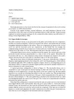
Figure 1.4: A Doppler ground speed sensor inclined
at an angle  as shown measures the velocity
component
V
of true ground speed
V
(adapted from
DA
[Schultz, 1993]).
1.2 Doppler Sensors
The rotational displacement sensors discussed above derive navigation parameters directly from
wheel rotation, and are thus subject to problems arising from slippage, tread wear, and/or improper
tire inflation. In certain applications, Doppler and inertial navigation techniques are sometimes
employed to reduce the effects of such error sources.
Doppler navigation systems are routinely employed in maritime and aeronautical applications to
yield velocity measurements with respect to the earth itself, thus eliminating dead-reckoning errors
introduced by unknown ocean or air currents. The principle of operation is based on the Doppler
shift in frequency observed when radiated energy reflects off a surface that is moving with respect
to the emitter. Maritime systems employ acoustical energy reflected from the ocean floor, while
airborne systems sense microwave RF energy bounced off the surface of the earth. Both
configurations typically involve an array of four transducers spaced 90 apart in azimuth and inclined
o
downward at a common angle with respect to the horizontal plane [Dunlap & Shufeldt, 1972].
Due to cost constraints and the reduced likelihood of transverse drift, most robotic implementa-
tions employ but a single forward-looking transducer to measure ground speed in the direction of
travel. Similar configurations are sometimes used in the agricultural industry, where tire slippage in

soft freshly plowed dirt can seriously interfere with the need to release seed or fertilizer at a rate
commensurate with vehicle advance. The M113-based Ground Surveillance Vehicle [Harmon,
1986] employed an off-the-shelf unit of this type manufactured by John Deere to compensate for
track slippage.
The microwave radar sensor is aimed downward at a prescribed angle (typically 45 ) to sense
o
ground movement as shown in Fig. 1.4. Actual ground speed V is derived from the measured
A
velocity V according to the following equation [Schultz, 1993]:
D

where
V = actual ground velocity along path
A
V = measured Doppler velocity
D
" = angle of declination
c = speed of light
F = observed Doppler shift frequency
D
F = transmitted frequency.
O
Errors in detecting true ground speed arise
due to side-lobe interference, vertical velocity
components introduced by vehicle reaction to
road surface anomalies, and uncertainties in the
actual angle of incidence due to the finite width
Part I: Sensors for Mobile Robot Positioning Chapter 1: Sensors for Dead Reckoning
Page 13
Fig. 1.5: The Trak-Star Ultrasonic

Speed Sensor is based on the
Doppler effect. This device is primarily
targeted at the agricultural market
Reproduced from [Micro-Trak].
Specification Value
Speed range 0-40 MPH (17.7 m/s)
Speed Resolution 0.04 MPH (1.8 cm/s)
Accuracy ±1.5%+0.04 MPH
Transmit Frequency 62.5 KHz
Temperature range -20 F to 120 F
oo
Weight 3 lb
Power Requirements 12 Volt Amp
Table 1.1: Specifications for the Trak-Star Ultrasonic Speed
Sensor
of the beam. Byrne et al. [1992] point out another interesting scenario for potentially erroneous
operation, involving a stationary vehicle parked over a stream of water. The Doppler ground-speed
sensor in this case would misinterpret the relative motion between the stopped vehicle and the
running water as vehicle travel.
1.2.1 Micro-Trak Trak-Star Ultrasonic Speed Sensor
One commercially available speed sensor that is based on
Doppler speed measurements is the Trak-Star Ultrasonic
Speed Sensor [MICRO-TRAK]. This device, originally
designed for agricultural applications, costs $420. The manu-
facturer claims that this is the most accurate Doppler speed
sensor available. The technical specifications are listed in
Table 1.1.
1.2.2 Other Doppler Effect Systems
Harmon [1986] describes a system using a Doppler effect
sensor, and a Doppler effect system based on radar is de-

scribed in [Patent 1].
Another Doppler Effect device is the Monitor 1000, a
distance and speed monitor for runners. This device was
temporarily marketed by the sporting goods manufacturer [NIKE]. The Monitor 1000 was worn by
the runner like a front-mounted fanny pack. The small and lightweight device used ultrasound as the
carrier, and was said to have an accuracy of 2-5%, depending on the ground characteristics. The
manufacturer of the Monitor 1000 is Applied Design Laboratories [ADL]. A microwave radar
Doppler effect distance sensor has also been developed by ADL. This radar sensor is a prototype
and is not commercially available. However, it differs from the Monitor 1000 only in its use of a
radar sensor head as opposed to the ultrasonic sensor head used by the Monitor 1000. The prototype
radar sensor measures 15×10×5 cm (6"×4"×2"), weighs 250 gr, and consumes 0.9 W.
1.3 Typical Mobility Config-
urations
The accuracy of odometry mea-
surements for dead-reckoning is to
a great extent a direct function of
the kinematic design of a vehicle.
Because of this close relation be-
tween kinematic design and posi-
tioning accuracy, one must consider
deadre05.ds4, .wmf, 10/19/94
Part I: Sensors for Mobile Robot Positioning Chapter 1: Sensors for Dead Reckoning
Page 14
Figure 1.6: A typical differential-drive mobile robot
(bottom view).
the kinematic design closely before attempting to improve dead-reckoning accuracy. For this reason,
we will briefly discuss some of the more popular vehicle designs in the following sections. In Part
II of this report, we will discuss some recently developed methods for reducing dead-reckoning
errors (or the feasibility of doing so) for some of these vehicle designs.
1.3.1 Differential Drive

Figure 1.6 shows a typical differential drive
mobile robot, the LabMate platform, manufac-
tured by [TRC]. In this design incremental
encoders are mounted onto the two drive motors
to count the wheel revolutions. The robot can
perform dead reckoning by using simple geomet-
ric equations to compute the momentary position
of the vehicle relative to a known starting posi-
tion. For completeness, we rewrite the well-
known equations for dead-reckoning below
(also, see [Klarer, 1988; Crowley and Reignier,
1992]).
Suppose that at sampling interval I the left and right wheel encoders show a pulse increment of
N and N , respectively. Suppose further that
LR
c = BD /nC
mne
where
c = Conversion factor that translates encoder pulses into linear wheel displacement
m
D = Nominal wheel diameter (in mm)
n
C = Encoder resolution (in pulses per revolution)
e
n = Gear ratio of the reduction gear between the motor (where the encoder is attached) and the
drive wheel.
We can compute the incremental travel distance for the left and right wheel, )U and )U ,
L,i R,i
according to
)U = c N

L/R, I m L/R, I
and the incremental linear displacement of the robot's centerpoint C, denoted )U , according to
i
)U = ()U + )U )/2
iRL
Next, we compute the robot's incremental change of orientation
)2 = ()U - )U )/b
iRL
Part I: Sensors for Mobile Robot Positioning Chapter 1: Sensors for Dead Reckoning
Page 15
where b is the wheelbase of the vehicle, ideally measured as the distance between the two contact
points between the wheels and the floor.
The robot's new relative orientation 2 can be computed from
i
2 = 2 + )2
i i-1 i
and the relative position of the centerpoint is
x = x + )U cos2
i i-1 i i
y = y + )Usin2
i i-1 i i
where
x , y - relative position of the robot's centerpoint c at instant I.
ii
1.3.2 Tricycle Drive
Tricycle drive configurations (see Fig. 1.7) employing a single driven front wheel and two passive
rear wheels (or vice versa) are fairly common in AGV applications because of their inherent
simplicity. For odometry instrumentation in the form of a steering angle encoder, the dead reckoning
solution is equivalent to that of an Ackerman-steered vehicle, where the steerable wheel replaces
the imaginary center wheel discussed in Section 1.3.3. Alternatively, if rear-axle differential

odometry is used to determine heading, the solution is identical to the differential-drive configuration
discussed in Section 1.3.1.
One problem associated with the tricycle drive configuration is the vehicle’s center of gravity
tends to move away from the front wheel when traversing up an incline, causing a loss of traction.
As in the case of Ackerman-steered designs, some surface damage and induced heading errors are
possible when actuating the steering while the platform is not moving.
Y
X
Steerable Driven Wheel
d
Passive Wheels
l
θ
Y
X
d
l
o
SA
i
θθ
θ
P
2
P
1
cot cotθθ
io
d
l

−=
Part I: Sensors for Mobile Robot Positioning Chapter 1: Sensors for Dead Reckoning
Page 16
Figure 1.7: Tricycle-drive configurations employing a steerable driven wheel and two
passive trailing wheels can derive heading information directly from a steering angle
encoder or indirectly from differential odometry [Everett, 1995].
Figure 1.8: In an Ackerman-steered vehicle, the extended axes for
all wheels intersect in a common point (adapted from [Byrne et al,
1992]).
1.3.3 Ackerman Steering
Used almost exclusively in the automotive industry, Ackerman steering is designed to ensure the
inside front wheel is rotated to a slightly sharper angle than the outside wheel when turning, thereby
eliminating geometrically induced tire slippage. As seen in Fig. 1.8, the extended axes for the two
front wheels intersect in a common point that lies on the extended axis of the rear axle. The locus
of points traced along the ground by the center of each tire is thus a set of concentric arcs about this
centerpoint of rotation P , and (ignoring for the moment any centrifugal accelerations) all
1
instantaneous velocity vectors will subse-
quently be tangential to these arcs. Such a
steering geometry is said to satisfy the
Ackerman equation [Byrne et al, 1992]:
where
2 = relative steering angle of inner wheel
i
2 = relative steering angle of outer wheel
o
l = longitudinal wheel separation
d = lateral wheel separation.
cot cotθθ
SA i

d
l
=+
2
cot cotθθ
SA o
d
l
=−
2
Part I: Sensors for Mobile Robot Positioning Chapter 1: Sensors for Dead Reckoning
Page 17
For the sake of convenience, the vehicle steering angle 2 can be thought of as the angle (relative
SA
to vehicle heading) associated with an imaginary center wheel located at a reference point P as
2
shown in the figure above. 2 can be expressed in terms of either the inside or outside steering
SA
angles (2 or 2 ) as follows [Byrne et al, 1992]:
io

or, alternatively,
.
Ackerman steering provides a fairly accurate dead-reckoning solution while supporting the
traction and ground clearance needs of all-terrain operation, and is generally the method of choice
for outdoor autonomous vehicles. Associated drive implementations typically employ a gasoline or
diesel engine coupled to a manual or automatic transmission, with power applied to four wheels
through a transfer case, differential, and a series of universal joints. A representative example is
seen in the HMMWV-based prototype of the USMC Tell-operated Vehicle (TOV) Program [Aviles
et al, 1990]. From a military perspective, the use of existing-inventory equipment of this type

simplifies some of the logistics problems associated with vehicle maintenance. In addition, reliability
of the drive components is high due to the inherited stability of a proven power train. (Significant
interface problems can be encountered, however, in retrofitting off-the-shelf vehicles intended for
human drivers to accommodate remote or computer control).
1.3.4 Synchro-Drive
An innovative configuration known as synchro-drive features three or more wheels (Fig. 1.9)
mechanically coupled in such a way that all rotate in the same direction at the same speed, and
similarly pivot in unison about their respective steering axes when executing a turn. This drive and
steering “synchronization” results in improved dead-reckoning accuracy through reduced slippage,
since all wheels generate equal and parallel force vectors at all times.
The required mechanical synchronization can be accomplished in a number of ways, the most
common being chain, belt, or gear drive. Carnegie Mellon University has implemented an
electronically synchronized version on one of their Rover series robots, with dedicated drive motors
for each of the three wheels. Chain- and belt-drive configurations experience some degradation in
steering accuracy and alignment due to uneven distribution of slack, which varies as a function of
loading and direction of rotation. In addition, whenever chains (or timing belts) are tightened to
reduce such slack, the individual wheels must be realigned. These problems are eliminated with a
completely enclosed gear-drive approach. An enclosed gear train also significantly reduces noise
as well as particulate generation, the latter being very important in clean-room applications.