- Trang chủ >>
- Khoa Học Tự Nhiên >>
- Vật lý
Path integrals in physics, vol 2 QFT, statistical physics and modern applications chaichian m , demichev a
Bạn đang xem bản rút gọn của tài liệu. Xem và tải ngay bản đầy đủ của tài liệu tại đây (2.56 MB, 355 trang )
Path Integrals in Physics
Vo l um e I I
Quantum Field Theory, Statistical Physics and
other Modern Applications
Path Integrals in Physics
Volume II
Quantum Field Theory, Statistical Physics
and other Modern Applications
M Chaichian
Department of Physics, University of Helsinki
and
Helsinki Institute of Physics, Finland
and
ADemichev
Institute of Nuclear Physics, Moscow State University, Russia
Institute of Physics Publishing
Bristol and Philadelphia
c
IOP Publishing Ltd 2001
All rights reserved. No part of this publication may be reproduced, stored in a retrieval system or
transmitted in any form or by any means, electronic, mechanical, photocopying, recording or otherwise,
without the prior permission of the publisher. Multiple copying is permitted in accordance with the
terms of licences issued by the Copyright Licensing Agency under the terms of its agreement with the
Committee of Vice-Chancellors and Principals.
British Library Cataloguing-in-Publication Data
A catalogue record for this book is available from the British Library.
ISBN 0 7503 0801 X (Vol. I)
0 7503 0802 8 (Vol. II)
0 7503 0713 7 (2 Vol. set)
Library of Congress Cataloging-in-Publication Data are available
Commissioning Editor: James Revill
Production Editor: Simon Laurenson
Production Control: Sarah Plenty
Cover Design: Victoria Le Billon
Marketing Executive: Colin Fenton
Published by Institute of Physics Publishing, wholly owned by The Institute of Physics, London
Institute of Physics Publishing, Dirac House, Temple Back, Bristol BS1 6BE, UK
US Office: Institute of Physics Publishing, The Public Ledger Building, Suite 1035, 150 South
Independence Mall West, Philadelphia, PA 19106, USA
Typeset in T
E
X using the IOP Bookmaker Macros
Printed in the UK by Bookcraft, Midsomer Norton, Bath
Contents
Preface to volume II ix
3 Quantum field theory: the path-integral approach 1
3.1 Path-integral formulation of the simplest quantum field theories 2
3.1.1 Systems with an infinite number of degrees of freedom and quantum field theory 2
3.1.2 Path-integral representation for transition amplitudes in quantum field theories 14
3.1.3 Spinor fields: quantization via path integrals over Grassmann variables 21
3.1.4 Perturbation expansion in quantum field theory in the path-integral approach 22
3.1.5 Generating functionals for Green functions and an introduction to functional
methods in quantum field theory 27
3.1.6 Problems 38
3.2 Path-integral quantization of gauge-field theories 49
3.2.1 Gauge-invariant Lagrangians 50
3.2.2 Constrained Hamiltonian systems and their path-integral quantization 54
3.2.3 Yang–Mills fields: constrained systems with an infinite number of degrees of
freedom 60
3.2.4 Path-integral quantization of Yang–Mills theories 64
3.2.5 Covariant generating functional in the Yang–Mills theory 67
3.2.6 Covariant perturbation theory for Yang–Mills models 73
3.2.7 Higher-order perturbation theory and a sketch of the renormalization procedure
for Yang–Mills theories 80
3.2.8 Spontaneous symmetry-breaking of gauge invariance and a brief look at the
standard model of particle interactions 88
3.2.9 Problems 98
3.3 Non-perturbative methods for the analysis of quantum field models in the path-integral
approach 101
3.3.1 Rearrangements and partial summations of perturbation expansions: the 1/N-
expansion and separate integration over high and low frequency modes 101
3.3.2 Semiclassical approximationin quantum field theory and extendedobjects (solitons)110
3.3.3 Semiclassical approximation and quantum tunneling (instantons) 120
3.3.4 Path-integral calculation of quantum anomalies 130
3.3.5 Path-integral solution of the polaron problem 137
3.3.6 Problems 144
3.4 Path integrals in the theory of gravitation, cosmology and string theory: advanced
applications of path integrals 149
vi
Contents
3.4.1 Path-integral quantization of a gravitational field in an asymptotically flat
spacetime and the corresponding perturbation theory 149
3.4.2 Path integrals in spatially homogeneous cosmological models 154
3.4.3 Path-integral calculation of the topology-changetransitions in (2+1)-dimensional
gravity 160
3.4.4 Hawking’s path-integral derivation of the partition function for black holes 166
3.4.5 Path integrals for relativistic point particles and in the string theory 174
3.4.6 Quantum field theory on non-commutative spacetimes and path integrals 185
4 Path integrals in statistical physics 194
4.1 Basic concepts of statistical physics 195
4.2 Path integrals in classical statistical mechanics 200
4.3 Path integrals for indistinguishable particles in quantum mechanics 205
4.3.1 Permutations and transition amplitudes 206
4.3.2 Path-integral formalism for coupled identical oscillators 210
4.3.3 Path integrals and parastatistics 216
4.3.4 Problems 221
4.4 Field theory at non-zero temperature 223
4.4.1 Non-relativistic field theory at non-zero temperature and the diagram technique 223
4.4.2 Euclidean-time relativistic field theory at non-zero temperature 226
4.4.3 Real-time formulation of field theory at non-zero temperature 233
4.4.4 Path integrals in the theory of critical phenomena 238
4.4.5 Quantum field theory at finite energy 245
4.4.6 Problems 252
4.5 Superfluidity, superconductivity,non-equilibrium quantum statistics and the path-integral
technique 257
4.5.1 Perturbation theory for superfluid Bose systems 258
4.5.2 Perturbation theory for superconducting Fermi systems 261
4.5.3 Non-equilibrium quantum statistics and the process of condensation of an ideal
Bose gas 263
4.5.4 Problems 277
4.6 Non-equilibrium statistical physics in the path-integral formalism and stochastic
quantization 280
4.6.1 A zero-dimensional model: calculation of usual integrals by the method of
‘stochastic quantization’ 281
4.6.2 Real-time quantum mechanics within the stochastic quantization scheme 284
4.6.3 Stochastic quantization of field theories 288
4.6.4 Problems 293
4.7 Path-integral formalism and lattice systems 295
4.7.1 Ising model as an example of genuine discrete physical systems 296
4.7.2 Lattice gauge theory 302
4.7.3 Problems 308
Supplements 311
I Finite-dimensional Gaussian integrals 311
II Table of some exactly solved Wiener path integrals 313
III Feynman rules 316
IV Short glossary of selected notions from the theory of Lie groups and algebras 316
Contents
vii
V Some basic facts about differential Riemann geometry 325
VI Supersymmetry in quantum mechanics 329
Bibliography 332
Index 337
Preface to volume II
In the second volume of this book (chapters 3 and 4) we proceed to discuss path-integral applications
for the study of systems with an infinite number of degrees of freedom. An appropriate description of
such systems requires the use of second quantization, and hence, field theoretical methods. The starting
point will be the quantum-mechanical phase-space path integrals studied in volume I, which we suitably
generalize for the quantization of field theories.
One of the central topicsof chapter 3 is the formulation of the celebrated Feynman diagram technique
for the perturbation expansion in the case of field theories with constraints (gauge-field theories),
which describe all the fundamental interactions in elementary particle physics. However, the important
applications of path integrals in quantum field theory go far beyond just a convenient derivation of the
perturbation theory rules. We shall consider, in this volume, various modern non-perturbativemethods for
calculations in field theory, such as variational methods, the description of topologically non-trivial field
configurations, the quantization of extended objects (solitons and instantons), the 1/N-expansion and the
calculation of quantum anomalies. In addition, the last section of chapter 3 contains elements of some
advanced and currently developing applications of the path-integral technique in the theory of quantum
gravity, cosmology, black holes and in string theory.
For a successful reading of the main part of chapter 3, it is helpful to have some acquaintance with
a standard course of quantum field theory, at least at a very elementary level. However, some parts
(e.g., quantization of extended objects, applications in gravitation and string theories) are necessarily
more fragmentary and presented without much detail. Therefore, their complete understanding can be
achieved only by rather experienced readers or by further consultation of the literature to which we
refer. At the same time, we have tried to present the material in such a form that even those readers
not fully prepared for this part could get an idea about these modern and fascinating applications of path
integration.
As we stressed in volume I, one of the most attractive features of the path-integral approach is its
universality. This means it can be applied without crucial modifications to statistical (both classical
and quantum) systems. We discuss how to incorporate the statistical properties into the path-integral
formalism for the study of many-particle systems in chapter 4. Besides the basic principles of path-
integral calculations for systems of indistinguishable particles, chapter 4 contains a discussion of various
problems in modern statistical physics (such as the analysis of critical phenomena, calculations in field
theory at non-zero temperature or at fixed energy, as well as the study of non-equilibrium systems and
the phenomena of superfluidity and superconductivity). Therefore, to be tractable in a single book,
these examples contain some simplifications and the material is presented in a more fragmentary style
in comparison with chapters 1 and 2 (volume I). Nevertheless, we have again tried to make the text as
ix
x
Preface to volume II
self-contained as possible, so that all the crucial points are covered. The reader will find references to the
appropriate literature for further details.
Masud Chaichian, Andrei Demichev
Helsinki, Moscow
December 2000
Chapter 3
Quantum field theory: the path-integral approach
So far, we have been discussing systems containing only one or, at most, a few particles. However,
the method of path integrals readily generalizes to systems with many and even an arbitrary number of
degrees of freedom. Thus in this chapter we shall consider one more infinite limit related to path integrals
and discuss applications of the latter to systems with an infinite number of degrees of freedom. In other
words, we shall derive path-integral representations for different objects in quantum field theory (QFT).
Of course, this is nothing other than quantum mechanics for systems with an arbitrary or non-conserved
number of excitations (particles or quasiparticles). Therefore, the starting point for us is the quantum-
mechanical phase-space path integrals studied in chapter 2. In most practical applications in QFT, these
path integrals can be reduced to the Feynman path integrals over the corresponding configuration spaces
by integrating over momenta. This is especially important for relativistic theories where this transition
allows us to keep relativistic invariance of all expressions explicitly.
Apparently, the most important result of path-integral applications in QFT is the formulation of the
celebrated Feynman rules for perturbation expansion in QFT with constraints, i.e. in gauge-field theories
which describe all the fundamental interactions of elementary particles. In fact, Feynman derived his
important rules (Feynman 1948, 1950) (in quantum electrodynamics (QED)) just using the path-integral
approach! Later, these rules (graphically expressed in terms of Feynman diagrams) were rederived in
terms of the standard operator approach. But the appearanceof more complicated non-Abelian gauge-field
theories (which describe weak, strong and gravitational interactions) again brought much attention to the
path-integral method which had proved to be much more suitable in this case than the operator approach,
because the latter faces considerable combinatorial and other technical problems in the derivation of the
Feynman rules. In fact, it is this success that attracted wide attention to the path-integral formalism in
QFT and in quantum mechanics in general.
Further development of the path-integral formalism in QFT has led to results far beyond the
convenientderivation of perturbation theory rules. In particular, it has resulted in various non-perturbative
approximations for calculations in field theoretical models, variational methods, the description of
topologically non-trivial field configurations, the discovery of the so-called BRST (Becchi–Rouet–Stora–
Tyutin) symmetry in gauge QFT, clarification of the relation between quantization and the theory of
stochastic processes, the most natural formulationof string theory which is believed to be the most realistic
candidate for a ‘theory of everything’, etc.
In the first section of this chapter, we consider path-integral quantization of the simplest field theories,
including scalar and spinor fields. We derive the path-integral expression for the generating functional
of the Green functions and develop the perturbation theory for their calculation. In section 3.2, after
an introduction to the quantization of quantum-mechanical systems with constraints, we proceed to the
path-integral description of gauge theories. We derive the covariant generating functional and covariant
1
2
Quantum field theory: the path-integral approach
perturbation expansion for Yang–Mills theories with exact and spontaneously broken gauge symmetry,
including the realistic standard model of electroweak interactions and quantum chromodynamics (QCD),
which is the gauge theory of strong interactions.
In section 3.3, we present non-perturbative methods and results in QFT based on the path-
integral approach. They include 1/N-expansion, separate integration over different Fourier modes
(with appropriate approximations for different frequency ranges), semiclassical, in particular instanton,
calculations and the quantization of extended objects (solitons), the analysis and calculation of quantum
anomalies in the framework of the path integral and the Feynman variational method in non-relativistic
field theory (on the example of the so-called polaron problem).
Section 3.4 contains some advanced applications of path-integraltechniquesin the theoryof quantum
gravity, cosmology, black holes and string theory. Reading this section requires knowledge of the basic
facts and notions from Einstein’s general relativity and the differential geometry of Riemann manifolds
(some of these are collected in supplement V).
We must stress that, although we intended to make the text as self-contained as possible, this chapter
by no means can be considered as a comprehensive introduction to such a versatile subject as QFT. We
mostly consider those aspects of the theory which have their natural and simple description in terms of
path integrals. Other important topics can be found in the extensive literature on the subject (see e.g.,
Wentzel (1949), Bogoliubov and Shirkov (1959), Schweber (1961), Bjorken and Drell (1965), Itzykson
and Zuber (1980), Chaichian and Nelipa (1984), Greiner and Reinhardt (1989), Peskin and Schroeder
(1995) and Weinberg (1995, 1996, 2000)).
3.1 Path-integral formulation of the simplest quantum field theories
After a short exposition of the postulates and main facts from conventional field theory, we present the
path-integral formulation of the simplest models: a single scalar field and a fermionic field. The latter
requires path integration over the Grassmann variables considered at the end of chapter 2. Then we
consider the perturbation expansion and generating functional for these simple theories which serve as
introductory examples for the study of the realistic models presented in the next section.
3.1.1 Systems with an infinite number of degrees of freedom and quantum field theory
There are various formulations of quantum field theory, differing in the form of presentation
of the basic quantities, namely transition amplitudes. In the operator approach, the transition
amplitudes are expressed as the vacuum expectation value of an appropriate product of particle
creation and annihilation operators. These operators obey certain commutation relations
(generalization of the standard canonical commutation relations to a system with an infinite
number of degrees of freedom). Another formulation is based on expressing the transition
amplitudes in terms of path integrals over the fields. In studying the gauge fields, the path-
integral formalism has proven to be the most convenient. However, for an easier understanding
of the subject we shall start by considering unconstrained fields and then proceed to gauge-field
theories (i.e. field theories with constraints).
Let us consider, as a starting example, a single scalar field. From the viewpoint of
Hamiltonian dynamics, a field is a system with an infinitely large number of degrees of freedom,
for the field is characterized by a generalized coordinate ϕ(x) and a generalized momentum π(x)
at each space point x ∈
d
.
It is worth making the following remark. If we were intending to provide an introduction to
the very subject of quantum field theory, it would be pedagogically more reasonable to start
from non-relativistic many-body problems and the corresponding non-relativistic quantum field
Path-integral formulation of the simplest quantum field theories
3
aaa
q
k−1
q
k−2
q
k
q
k+1
··· ···
equilibrium
positions
Figure 3.1. Vibrating chain of coupled oscillators; the distances between the equilibrium positions of the particles
are equal to some fixed value a, the displacements of the particles from the equilibrium positions are the dynamical
variables and are denoted by q
k
(k = 1, ,K).
theories, as they are the closest generalization of one (or at most a few) particle problems in
quantum mechanics. However, the area of the most fruitful applications of non-relativistic field
theories is the physics of quantum statistical systems, in general with non-zero temperature.
Path integrals for statistical systems have some peculiarities (in particular, the corresponding
trajectories may have a rather specific meaning, one which is quite different from that in quantum
mechanics). Therefore, we postpone discussion of such systems until the next chapter and
now proceed to consider path-integral formulation of quantum field theories at zero temperature
which finds its main application in the description of the
relativistic
quantum mechanics of
elementary particles. In this chapter, we shall encounter only one example of a non-relativistic
field theoretical model which describes the behaviour of an electron inside a crystal (the so-
called
polaron problem
).
♦Quantum fields as an infinite number of degrees of freedom limit of systems of coupled oscillators
In order to approach the consideration of systems with an infinite number of degrees of
freedom (quantum fields) we start from a chain of K coupled oscillators with equal masses
and frequencies, in the framework of ordinary quantum mechanics (see figure 3.1).
The Hamiltonian of such a system has the form
H =
K
k=1
1
2
[p
2
k
+
2
(q
k
− q
k+1
)
2
+
2
0
q
2
k
] (3.1.1)
where p
k
, q
k
(k = 1, ,K) are the canonical variables (momentum and position) of the kth
oscillator and the equations of motion read:
˙q
k
= p
k
˙p
k
=
2
(q
k+1
+ q
k−1
− 2q
k
) −
2
0
q
k
(3.1.2)
or, written only in terms of coordinates,
¨q
k
=
2
(q
k+1
+ q
k−1
− 2q
k
) −
2
0
q
k
. (3.1.3)
The frequency
0
defines the potential energy of an oscillator due to a shift from its equilibrium
position and the frequency defines the interaction of an oscillator with its neighbours. Since
we shall use this model as a starting point for the introduction of quantum fields, a concrete
4
Quantum field theory: the path-integral approach
value of the particle masses in (3.1.1) is not important and for convenience we have put it equal
to unity (cf (2.1.42)). Besides, as is usual in relativistic quantum field theory, we use units such
that
= 1.
The equations of motion must be accompanied by some boundary conditions. Since we
are going to pass later to systems in infinite volumes (of infinite sizes), the actual form of
the boundary conditions should not have a crucial influence on the behaviour of the systems.
Therefore, we can choose them freely and the most convenient one is the periodic condition:
q
k+K
= q
k
. (3.1.4)
After the quantization, the canonical variables become operators with the following
canonical commutation relations:
[q
k
, p
l
]=iδ
kl
[q
k
,q
l
]=[p
k
, p
l
]=0 κ, l = 1, ,K.
(3.1.5)
In order to find the eigenvalues of the corresponding quantum Hamiltonian
H =
K
k=1
1
2
[p
2
k
+
2
(q
k
−q
k+1
)
2
+
2
0
q
2
k
] (3.1.6)
it is helpful to introduce new variables (the so-called
normal coordinates
)
Q
r
,
P
r
via the discrete
Fourier transform:
q
k
=
1
√
K
K/2
r=−K/2+1
Q
r
e
i2πrk/K
p
k
=
1
√
K
K/2
r=−K/2+1
P
r
e
−i2πrk/K
(3.1.7)
with the analogous commutation relations
[
Q
r
,
P
s
]=iδ
rs
[
Q
r
,
Q
s
]=[
P
r
,
P
s
]=0
(3.1.8)
where r and s are integers from the interval [−K/2 +1, K/2]. It is easy to verify that the normal
coordinates also satisfy the periodic conditions:
Q
−K/2
=
Q
K/2
and
P
−K/2
=
P
K/2
, so that we
again have 2N independent variables (as in the case of q
k
, p
k
). This restriction, as well as the
range of the summations in (3.1.7), follows from the periodic boundary conditions (3.1.5). Since
q
k
, p
k
are Hermitian operators, the new operators satisfy the conditions
Q
†
k
=
Q
−k
P
†
k
=
P
−k
. (3.1.9)
The Kronecker symbol δ
ln
can be represented as the sum
K
k=1
e
i2πk(l−n)/K
= Kδ
ln
. (3.1.10)
Path-integral formulation of the simplest quantum field theories
5
This is an analog of the integral representation (1.1.22) for the δ-function, adapted to the
discrete finite lattice with a periodic boundary condition. Using this formula, we can invert the
transformation (3.1.7) of the dynamical variables:
Q
r
=
1
√
K
K
k=1
q
k
e
−i2πrk/K
P
r
=
1
√
K
K
k=1
p
k
e
i2πrk/K
.
(3.1.11)
In the normal coordinates Q
r
, P
r
the Hamiltonian (3.1.6) takes the simpler form
H =
1
2
K/2
r=−K/2+1
[
P
r
P
†
r
+ ω
2
r
Q
r
Q
†
r
] (3.1.12)
ω
2
r
≡
2
2sin
2πr
K
+
2
0
. (3.1.13)
Thus, in the normal coordinates we have K non-interacting oscillators and it is natural to
introduce the creation and annihilation operators (cf (2.1.47), taking into account that Q
r
, P
r
now are not Hermitian operators):
a
r
=
1
√
ω
r
(ω
r
Q
r
+ i
P
†
r
)
a
†
r
=
1
√
ω
r
(ω
r
Q
†
r
− i
P
r
)
(3.1.14)
(note that a
−r
= a
†
r
). The commutation relations for a
r
, a
†
r
are derived from (3.1.8) with the
expected result:
[a
r
,a
†
s
]=δ
rs
[a
r
,a
s
]=[a
†
r
,a
†
s
]=0.
(3.1.15)
In terms of these operators, the Hamiltonian (3.1.12) reads as
H =
K/2
r=−K/2+1
ω
r
(a
†
r
a
r
+
1
2
). (3.1.16)
Eigenstates of the Hamiltonian written in the latter form can be constructed in the standard way:
the state
|n
−K/2+1
, n
−K/2+2
, ,n
K/2
=
K/2
r=−K/2+1
1
√
n
r
!
(a
†
r
)
n
r
|0 (3.1.17)
is the Hamiltonian eigenstate with energy (eigenvalue)
E = E
0
+
r
n
r
ω
r
. (3.1.18)
6
Quantum field theory: the path-integral approach
The state |0 in (3.1.17) has the lowest energy:
E
0
=
r
ω
r
2
(3.1.19)
and is defined by the conditions
a
r
|0=0 r =−K/2 +1, ,K/2. (3.1.20)
Let us consider the continuous limit for a chain of coupled oscillators K →∞, a → 0,with
a finite value of the product aK ≡ L. Technically, this corresponds to the following substitutions:
q
k
−→
q(x)
√
a
k
−→
1
a
L
0
dx −→
v
a
(3.1.21)
and Hamiltonian (3.1.1) takes the following form in the limit
H =
L
0
dx
1
2
p
2
(x, t) +v
2
∂q
∂x
2
+
2
0
q
2
(x, t)
. (3.1.22)
Now the degrees of freedom of the system are ‘numbered’ by the continuous variable x.
However, for a finite length L, the normal coordinates Q
r
, P
r
are still countable:
q(x) =
1
√
L
∞
r=−∞
e
i2πr/L
Q
r
p(x) =
1
√
L
∞
r=−∞
e
i2πr/L
P
r
(3.1.23)
though the index r is now an arbitrary unbounded integer. The quantum Hamiltonian can be
cast again into the form (3.1.12) or (3.1.16):
H =
1
2
∞
r=−∞
(
P
r
P
†
r
+ ω
2
r
Q
r
Q
†
r
)
=
∞
r=−∞
ω
r
(a
†
r
a
r
+
1
2
) (3.1.24)
ω
2
r
= v
2
k
2
+
2
0
k ≡
2πr
L
(3.1.25)
with the only difference begin that the sums run over all integers. The eigenstates and
eigenvalues of this Hamiltonian are given by (3.1.17)–(3.1.20). The essentially new feature
of this system with an
infinite
number of degrees of freedom (i.e. after the transition K →∞)is
that the energy (3.1.19) of the lowest eigenstate |0 becomes
infinite
. We can circumvent this
difficulty by redefining the Hamiltonian as follows:
H −→
H − E
0
=
1
2
∞
r=−∞
ω
r
a
†
r
a
r
(3.1.26)
Path-integral formulation of the simplest quantum field theories
7
i.e. counting the energy with respect to the lowest state |0. This is the simplest example of the
so-called renormalizations in quantum field theory.
All the considerations outlined here can easily be generalized to higher-dimensional lattices
and corresponding higher-dimensional spaces in the continuous limit. In the latter case, the
dynamical variables depend on (are labeled by) d-dimensional vectors:
q(x, t) −→ ˆϕ(x, t) p(x, t) −→ ˆπ(x, t) x ∈
d
(3.1.27)
so that we have arrived in this way at the notion of the
quantum field in the
(d + 1)
-dimensional
spacetime
. Note that the straightforward generalization of the coupled oscillator model
previously considered in the one-dimensional space leads to the
vector fields
ˆϕ(x, t), ˆπ(x, t)
because the displacements and momenta of oscillators in d-dimensional spaces are described
by vectors. However, if we assume that for some reason the displacements are confined to
one
direction, we obtain the physically important case of
scalar
quantum fields ˆϕ(x, t), ˆπ(x, t).
Hamiltonians for quantum fields in higher-dimensional spaces are the direct generalizations
of those for the one-dimensional case (cf (3.1.22)). In particular, for the most realistic three-
dimensional space, we have
H =
1
2
d
3
r [ˆπ
2
(r, t) +v
2
(∇ ˆϕ(r, t))
2
+
2
0
ˆϕ
2
(r, t)]. (3.1.28)
The operators of the quantum field ˆϕ(r, t) and the corresponding momentum ˆπ(r, t) satisfy the
canonical commutation relations at equal times:
[ˆϕ(r, t), ˆπ(r
, t)]=iδ
3
(r − r
)
[ˆϕ(r, t), ˆϕ(r
, t)]=[ˆπ(r, t), ˆπ(r
, t)]=0.
(3.1.29)
The three-dimensional periodic boundary conditions require the following equalities:
ϕ(x + L, y, z, t) = ϕ(x, y + L, z, t) = ϕ(x, y, z + L, t) = ϕ(x, y, z, t) (3.1.30)
and the corresponding Fourier transform,
ˆϕ(r, t) =
1
L
3/2
∞
k
x
,k
y
,k
z
=−∞
(2ω
k
)
−1/2
[e
i(k·r−ω
k
t)
a
k
+ e
−i(k·r−ω
k
t)
a
†
k
] (3.1.31)
k
x,y,z
=
2πl
x,y,z
L
(3.1.32)
ω
2
k
= v
2
k
2
+
2
0
(3.1.33)
allows us once again to convert (3.1.28) into the Hamiltonian for an infinite set of independent
oscillators:
H =
∞
l
x,y,z
=−∞
ω
k
(a
†
k
a
k
+
1
2
) (3.1.34)
with a
†
k
, a
k
being the creation and annihilation operators subjected to the following commutation
relations:
[a
k
,a
†
k
]=δ
kk
[a
k
,a
k
]=[a
†
k
,a
†
k
]=0.
(3.1.35)
8
Quantum field theory: the path-integral approach
The eigenstates and eigenvalues of this Hamiltonian again have the form (3.1.17)–(3.1.20),
so that the energy of a state |n
k
, n
k
2
, is completely defined by the set {n
k
1
} of
occupation
numbers
{n
k
}=n
k
1
, n
k
2
, (i.e. by powers of the creation operators on the right-hand side of
(3.1.17)):
E
{n
k
}
− E
0
=
i
n
k
i
ω
k
i
. (3.1.36)
Note that, if we put
v = c
0
= mc
2
(3.1.37)
where c is the speed of light and m is the mass of a particle, equation (3.1.33) exactly coincides
with the relativistic relation between energy, mass and momentum k of a particle. Hence,
expression (3.1.36) for the energy of the quantum field ϕ(x, t) can be interpreted as the sum
of energies of the set (defined by the occupation numbers {n
k
i
}) of free relativistic particles. To
simplify the formulae, we shall, in what follows, put the speed of light equal to unity, c = 1;the
latter can be achieved by an appropriate choice of units of measurement.
• Thus, we have obtained a remarkable result: a quantum field with the Hamiltonian (3.1.28)
(or (3.1.22)) and the choice of parameters as in (3.1.37) is equivalent to a system of
an arbitrary number of free relativistic particles. According to the commutation relations
(3.1.35), these particles obey Bose–Einstein statistics.
We have already mentioned the specific problems of quantum systems with an infinite
number of degrees of freedom, that is, the appearance of divergent expressions. One example
is the energy of ‘zero oscillations’ (3.1.19), which diverges for an infinite number of oscillators.
Another example is the expression for ‘zero fluctuations’ of the field ϕ(t, r), in other words for the
dispersion of the field in the lowest energy state:
(
|0
ˆϕ)
2
≡0|ˆϕ
2
|0
=
1
(2π)
3
d
3
k
1
2ω
k
=
1
(2π)
3
d
3
k
1
2
√
k
2
+ m
2
→∞. (3.1.38)
The reason for the infinite value of the fluctuation is related to the fact that ˆϕ,actingonan
arbitrary state with finite energy, gives a state with an infinite norm. Thus ˆϕ does not belong
to well-defined operators in the Hilbert space of states of the Hamiltonian under consideration.
Another way to express this fact is to say that ˆϕ is an operator-valued distribution (generalized
function). To construct a well-defined operator, we have to smear ˆϕ with an appropriate test
function, e.g., to consider the quantity
¯ϕ
λ
def
≡
1
(2πλ
2
)
3/2
d
3
r e
−r
2
/(2λ
2
)
ˆϕ(t, r) (3.1.39)
which can be interpreted as an average value of the field in the volume λ
3
around the point r.
The reader may check that the dispersion of ¯ϕ
λ
is finite:
0|¯ϕ
2
λ
|0≈
1
λ
3
√
λ
−2
+ m
2
(3.1.40)
(problem 3.1.1, page 38). The last expression shows that the smaller the volume λ
3
is, the
stronger the fluctuations of the field are. This fact, of course, is in full correspondence with the
quantum-mechanical uncertainty principle.
Path-integral formulation of the simplest quantum field theories
9
♦ Relativistic invariance of field theories and Minkowski space
To reveal explicitly the relativistic symmetry of the system described by the Hamiltonian (3.1.28)
with the parameters (3.1.37), we should pass to the Lagrangian formalism:
H[π(r, t), ϕ(r, t)]−→L[˙ϕ(r, t), ϕ(r, t)]
where L is the classical Lagrangian defined by the classical Hamiltonian H via the Legendre
transformation:
L[˙ϕ(r, t), ϕ(r, t)]=
d
3
r π(r, t) ˙ϕ(r, t) − H[π(r, t), ϕ(r, t)]. (3.1.41)
The momentum π on the right-hand side of (3.1.41) is assumed to be expressed through ˙ϕ, ϕ
with the help of the Hamiltonian equation of motion. In our case,
˙ϕ ={ϕ, H}=π (3.1.42)
(recall that {·, ·} is the Poisson bracket). Thus, the Lagrangian for the scalar field reads as
L(t) =
d
3
r
1
2
[˙ϕ
2
(r, t) −(∇ϕ(r, t))
2
− m
2
ϕ
2
(r, t)]. (3.1.43)
To demonstrate the invariance of the Lagrangian (3.1.43) with respect to transformations forming
relativistic kinematic groups, i.e. the
Lorentz
or
Poincar
´
e
groups, it is helpful to pass to
four-dimensional notation. Let us introduce the four-dimensional
Minkowski
space with the
coordinates:
x
µ
def
≡{t, r} µ = 0, 1, 2, 3 (3.1.44)
i.e.
x
0
= tx
i
= r
i
i = 1, 2, 3,
and the metric tensor
g
µν
= diag{1, −1, −1, −1} (3.1.45)
which defines the scalar product of vectors in the Minkowski space:
xy ≡ x
µ
y
µ
def
≡ x
µ
g
µν
y
ν
(repeating indices are assumed to be summed over). In particular, the squared vector in the
Minkowski space reads as
x
2
≡ (x
µ
)
2
= x
µ
g
µν
x
ν
= (x
0
)
2
− (x
1
)
2
− (x
2
)
2
− (x
3
)
2
= t
2
− r
2
= t
2
−r
2
1
−r
2
2
−r
2
3
(3.1.46)
or, for the infinitesimally small vector dx
µ
,
(dx
µ
)
2
= dx
µ
g
µν
dx
ν
= (dt)
2
− (dr)
2
. (3.1.47)
In the literature on relativistic field theory, it is common to drop boldface type for four-dimensional
vectors and we shall follow this custom. If the vector indices µ,ν, take, in some expressions,
10
Quantum field theory: the path-integral approach
only spacelike values 1, 2, 3, we shall denote them by Latin letters l, k, and use the following
shorthand notation:
A
l
B
l
=
3
l=1
A
l
B
l
where A
l
, B
l
are the spacelike components of some four-dimensional vectors A
µ
={A
0
, A
l
},
B
ν
={B
0
, B
l
}.
The Minkowski metric tensor g
µν
is invariant with respect to the transformations defined by
the pseudo-orthogonal 4 ×4 matrices
µ
ν
from the Lie group SO(1, 3), called the
Lorentz group
:
ρ
µ
g
ρσ
σ
ν
= g
µν
. (3.1.48)
This means that any scalar product in the Minkowski space is invariant with respect to the
Lorentz transformations. Moreover, the scalar products of vectors (recall that the latter are
expressed through the
differences
in the coordinates of two points) are also invariant with
respect to the four-dimensional translations forming the Abelian (commutative) group T
4
.In
particular, the reader can easily verify that dx
µ
g
µν
dx
ν
and (∂/∂ x
µ
)g
µν
(∂/∂ x
ν
), where g
µν
denotes the inverse matrix
g
µρ
g
ρν
= δ
µ
ν
are invariant with respect to both Lorentz ‘rotations’ as well as translations and, hence, with
respect to the complete
Poincar
´
e group
SO(1, 3)×⊃ T
4
.
We shall not go further into the details of relativistic kinematics, referring the reader to, e.g.,
Novozhilov (1975), Chaichian and Hagedorn (1998) or any textbook on quantum field theory (in
particular, those mentioned at the very beginning of this chapter).
To restore full equivalence between the time and space coordinates, it is useful to introduce
the Lagrangian density. This is nothing other than the integrand of (3.1.43), which, in four-
dimensional notation, takes the form
0
( ˙ϕ,ϕ) =
1
2
[g
µν
∂
µ
ϕ(x)∂
ν
ϕ(x) − m
2
ϕ
2
(x)]. (3.1.49)
The action for a scalar relativistic field and for the entire time line −∞ < x
0
< ∞ can now be
written as follows:
S
0
[ϕ]=
4
d
4
x
0
( ˙ϕ,ϕ). (3.1.50)
Taking into account the fact that the integration measure d
4
x = dx
0
dx
1
dx
2
dx
3
is invariant with
respect to the pseudo-orthogonal Lorentz transformations as well as with respect to translations,
we can readily check that action (3.1.50) is indeed Poincar
´
e invariant.
For a finite-time interval, t
0
< t ≡ x
0
< t
f
, the action reads as
S[ϕ]=
t
f
t
0
dx
0
L ≡
t
f
t
0
dx
0
3
dx
1
dx
2
dx
3
( ˙ϕ,ϕ). (3.1.51)
The equation of motion can now be derived from the extremality of action (3.1.51): δS = 0,
together with the boundary conditions that variations of the field at times t
0
and t
f
vanish:
δϕ(t
0
) = δϕ(t
f
) = 0, which result in the Euler–Lagrange equation
∂
∂t
δL
δ ˙ϕ
=
δL
δϕ
(3.1.52)
Path-integral formulation of the simplest quantum field theories
11
or
∂
∂t
∂
∂ ˙ϕ
=
∂
∂ϕ
− ∇
∂
∂∇ϕ
. (3.1.53)
For a free scalar field with the Lagrangian density (3.1.49), the Euler–Lagrange equation is
equivalent to the so-called
Klein–Gordon equation
:
(
+ m
2
)ϕ(x) = 0 (3.1.54)
where
def
≡ g
µν
∂
µ
∂
ν
≡
∂
2
∂t
2
− ∇
2
. (3.1.55)
In order to describe
interacting
particles, we have to add, to the Lagrangian density (3.1.49),
higher powers of the field ϕ(x):
(∂
µ
ϕ,ϕ) =
1
2
[g
µν
∂
µ
ϕ(x)∂
µ
ϕ(x) − m
2
ψ
2
(x)]−V(ϕ(x)). (3.1.56)
Here the function V(ϕ(x)) describes a field self-interaction. The equation of motion for ϕ now
becomes
(
+ m
2
)ϕ(x) =−
∂V (ϕ)
∂ϕ
. (3.1.57)
Most often, we shall consider a self-interaction of the form
V(ϕ(x)) =
g
4!
ϕ
4
(x) (3.1.58)
where g ∈
is called the
coupling constant
. In systems described by the Lagrangian (3.1.57)
and expressions similar to it (i.e. with interaction terms), particles (field excitations) can arise
and disappear, so that the total number of particles is
not a conserved quantity
.Thisisa
characteristic property of relativistic particle theory. Vice versa, it is clear that a system with an
arbitrary
number of particles definitely requires, for its description, a formalism with an infinite
number of degrees of freedom, i.e. the quantum field theory.
♦ Lagrangian for spin-
1
2
field, Dirac equation and operator quantization
Many well-established types of particle in nature (for example, electrons, positrons, quarks,
neutrinos) have half-integer spin J =
1
2
and obey Fermi statistics. Systems of such particles
are described by
spinor (fermion) quantum fields
satisfying
canonical anticommutation relations
(see any textbook on quantum field theory, e.g., Bogoliubov and Shirkov (1959), Bjorken and
Drell (1965) and Itzykson and Zuber (1980)).
A system of free relativistic spin-
1
2
fermions is described by a four-component complex field
ψ
α
(x), α = 1, ,4 and has the Lagrangian density
(x) =
¯
ψ(x)(i∂ − m)ψ(x) ≡
4
α,β=1
¯
ψ
α
(x)(i∂
αβ
− mδ
αβ
)ψ
β
(x) (3.1.59)
where we have introduced the standard notation: for any four-dimensional vector A
µ
,the
quantity A/ means
A/
def
≡ γ
µ
A
µ
= g
µν
γ
µ
A
ν
= γ
0
A
0
− γ · A (3.1.60)
12
Quantum field theory: the path-integral approach
and γ
µ
, µ = 0, 1, 2, 3 are the
Dirac matrices
satisfying the defining relations
γ
µ
γ
ν
+ γ
ν
γ
µ
= 2g
µν
1I
4
(3.1.61)
(1I
4
is the 4×4 unit matrix). In particular,∂ ≡ γ
µ
∂
µ
. One possible representation of the γ -matrices
has the form
γ
0
=
1I
2
0
0 −1I
2
γ
i
=
0 σ
i
−σ
i
0
i = 1, 2, 3. (3.1.62)
Here σ
i
are the Pauli matrices and 1I
2
is the 2 × 2 unit matrix. The
Dirac conjugate spinor
¯
ψ(x)
in (3.1.59) is defined as follows:
¯
ψ(x)
def
≡ ψ
†
(x)γ
0
or
¯
ψ
α
(x)
def
≡
4
β=1
ψ
†
β
(x)γ
0
βα
. (3.1.63)
Note that, as is usual in the literature on quantum field theory, we do not use special print for
either the γ -matrices or the Pauli matrices (similarly to four-dimensional vectors).
The extremality condition for the action with the density (3.1.59) (Euler equation) gives the
Dirac equation
for a spin-
1
2
field
(i∂ − m)ψ(x) = 0. (3.1.64)
The general form for the expansion of a solution of the Dirac equation (3.1.64) over plane waves
is the following:
ψ(t, r) =
1
(2π)
3/2
2
i=1
d
3
k [b
∗
i
(k)u
i
(k)e
ikx
+ c
i
(k)v
i
(k)e
−ikx
]
ψ
†
(t, r) =
1
(2π)
3/2
2
i=1
d
3
k [b
i
(k)u
†
i
(k)e
−ikx
+ c
∗
i
(k)v
†
i
(k)e
ikx
]
(3.1.65)
where k
0
= ω
k
≡
√
k
2
+ m
2
and u
i
(k), v
i
(k), i = 1, 2 comprise the complete set of orthonormal
solutions of the Dirac equation (in the momentum representation):
(k/ − m)u
i
(k)|
k
0
=
√
k
2
+m
2
= 0
(k/ +m)v
i
(k)|
k
0
=−
√
k
2
+m
2
= 0
so that, in fact, u
i
and v
i
are only functions of three-dimensional momentum k.
The orthogonality relations read as
¯v
i
(k)v
j
(k) ≡
n
α=1
( ¯v
i
(k))
α
(v
j
(k))
α
=−¯u
i
(k)u
j
(k) =
m
ω
k
δ
ij
v
†
i
(k)v
j
(k) = u
†
i
(k)u
j
(k) = δ
ij
(3.1.66)
¯u
i
(k)v
j
(k) = u
†
i
(k)v
j
(−k) = 0
Path-integral formulation of the simplest quantum field theories
13
and the completeness relations are
i
[(v
i
(k))
α
( ¯v
i
(k))
β
− (u
i
(k))
α
( ¯u
i
(k))
β
]=
m
ω
k
δ
αβ
i
(v
i
(k))
α
( ¯v
i
(k))
β
=
1
2ω
k
(k/
αβ
+ mδ
αβ
) (3.1.67)
i
(u
i
(k))
α
( ¯u
i
(k))
β
=
1
2ω
k
(k/
αβ
− mδ
αβ
).
The quantization procedure converts the amplitudes b
i
, b
∗
, c
i
, c
∗
i
into creation and annihilation
operators for fermionic particles. To take into account the Pauli principle, we have to impose
anticommutation relations
:
{
b
i
(k),
b
†
j
(k
)}=δ
ij
δ
3
(k − k
)
{c
i
(k),c
†
j
(k
)}=δ
ij
δ
3
(k − k
)
{
b
i
(k),
b
j
(k
)}={c
i
(k),c
j
(k
)}=0
{
b
†
i
(k),
b
†
j
(k
)}={c
†
i
(k),c
†
j
(k
)}=0
{
b
i
(k),c
j
(k
)}={
b
i
(k),c
†
j
(k
)}=0
{c
i
(k),
b
†
j
(k
)}={c
†
i
(k),
b
†
j
(k
)}=0.
(3.1.68)
From these relations, it is easy to derive the equal-time anticommutation relations for the fields
ˆ
ψ,
ˆ
ψ
†
:
{
ˆ
ψ
α
(t, r),
ˆ
ψ
†
β
(t, r
)}=δ
αβ
δ
3
(r − r
)
{
ˆ
ψ
α
(t, r),
ˆ
ψ
β
(t, r
)}=0 {
ˆ
ψ
†
α
(t, r),
ˆ
ψ
†
β
(t, r
)}=0.
(3.1.69)
Note that the canonical momentum π
α
conjugated to the field ψ
α
with respect to the Lagrangian
(3.1.59) is equal to iψ
†
α
:
π
α
≡
∂
∂
˙
ψ
α
= iψ
†
α
. (3.1.70)
Thus the commutation relations (3.1.69) are nothing other than the fermionic generalization of
the canonical commutation relations for (generalized) coordinates and conjugate momenta. The
corresponding Hamiltonian
H =
d
3
r (π
˙
ψ − )
( is the Lagrangian density (3.1.59)) in the quantum case can be written in terms of the
fermionic creation and annihilation operators:
H =
2
i=1
d
3
k ω
k
[
b
†
i
(k)
b
i
(k) −c
i
(k)c
†
i
(k)]. (3.1.71)
In order to make this Hamiltonian operator positive definite, we can use the anticommutation
relations (3.1.68) together with an infinite shift of the vacuum energy similarly to the bosonic
14
Quantum field theory: the path-integral approach
case (cf (3.1.26)):
H →
H − E
0
=
2
i=1
d
3
k ω
k
[
b
†
i
(k)
b
i
(k) +c
†
i
(k)c
i
(k)].
Sometimes this procedure of energy subtraction in the fermionic case is carried out by
invoking the qualitative concept of a Dirac ‘sea’, i.e. we assume that all negative-energy states
are occupied and real experimentally observable particles correspond to excitations of this
background state of the whole fermion system (see e.g., Bjorken and Drell (1965)).
3.1.2 Path-integral representation for transition amplitudes in quantum field theories
In the operator approach, there exist different representations for the canonical field operators ˆϕ(r) and
ˆπ(r) satisfying the commutation relations (3.1.29) or (3.1.69). For example, in the case of the scalar field
theory and in the coordinate representation, the vectors of the corresponding Hilbert space of states are
functionals [ϕ(r)] of the field ϕ(t, r) and the operator ˆϕ is diagonal:
ˆϕ(r)[ϕ(r)]=ϕ(r)[ϕ(r)]
ˆπ(r)[ϕ(r)]= −i
δ
δϕ(r)
[ϕ(r)].
Thus, when quantizing a field theory (in other words, a system with an infinite number of degrees of
freedom), even in the operator approach, we have to deal anyway with functionals, so that an application
of path (functional) integrals in this area is highly natural.
♦ Path integrals in scalar field theory
In fact, the introduction of quantum fields, presented in this section, as the limit of systems with a finite
number of degrees of freedom (coupled oscillators), allows us to write immediately an expression for
the corresponding transition amplitude (the quantum-mechanical propagator). Indeed, in the case of a
field theory, the space coordinates r ={x
1
, x
2
, x
3
} label the different degrees of freedom. For the lattice
approximation (with spacing a) in a finite volume L
3
, from which we started in this section, we have
simply a finite number K
3
of oscillators q
k
= ϕ(r
k
) (cf (3.1.21) and (3.1.27); generally speaking, we
have anharmonic oscillators because of the self-interaction term V(ϕ) in (3.1.56)). Therefore, we can
write the transition amplitude for the quantum fields as a direct generalization (infinite limit) of the path-
integral representation for propagatorsof quantum-mechanicalsystems with a finite number of degrees of
freedom obtained in chapter 2 (cf (2.2.9) and (2.2.21)):
ϕ(t, r), t|ϕ
0
(t
0
, r), t
0
=ϕ(r)|e
−i(t−t
0
)
H
|ϕ
0
(r)
= lim
L→∞
lim
K→∞
a→0
lim
N→∞
ε→0
K
k=1
N
j=1
∞
−∞
dϕ
j
(r
k
)
N+1
j=1
∞
−∞
dπ
j
(r
k
)
2π
×exp{iS
N
(π
i
(r
l
), ;ϕ
s
(r
l
), )} (3.1.72)
where the discrete-time and discrete-space approximated action S
N
depends on all π
i
(r
l
), i = 1, ,N +
1; l = 1, ,K and ϕ
s
(r
l
), s = 0, ,N + 1; l = 1, ,K variables (N is the number of time slices
and ε is the ‘distance’ between the time slices). In the case of Hamiltonian (3.1.28), the continuous limits
Path-integral formulation of the simplest quantum field theories
15
in (3.1.72) correspond to the following path integral:
ϕ(t, r), t|ϕ
0
(t
0
, r), t
0
=
{ϕ
0
(r),t
0
;ϕ(r),t}
ϕ(τ, r)
π(τ, r)
2π
exp
i
t
t
0
dτ
3
d
3
r
π(τ, r)∂
τ
ϕ(τ, r)
−
1
2
3
i=1
(∂
i
ϕ(τ, r))
2
−
1
2
m
2
ϕ
2
(τ, r) − V (ϕ(τ, r))
. (3.1.73)
Gaussian integration over the momenta π(τ, r) yields the Feynman path integral in the coordinate space:
ϕ(t, r), t|ϕ
0
(t
0
, r), t
0
=
−1
{ϕ
0
(r),t
0
;ϕ(r),t}
dτ
ϕ(τ, r) exp
i
t
t
0
dx
0
3
dx
1
dx
2
dx
3
(ϕ)
(3.1.74)
where the Lagrangian density
(ϕ) is defined in (3.1.56) and
−1
def
≡
π(x) exp
−
i
2
dxπ
2
(x)
(3.1.75)
is the normalization constant for expressing the transition amplitude via the Feynman (configuration) path
integral.
Expression (3.1.74) is almost invariant with respect to relativistic Poincar´e transformations. The
only source of non-invariance is the restriction of the time integral in the exponent to the finite interval
[t
0
, t]. However, it is necessary to point out that elementary particle experimentalists do not measure
probabilities directly related to amplitudes for transitions between eigenstates |ϕ(t
0
, r), t
0
and |ϕ(t, r), t
of the quantum field ˆϕ(τ, r), but rather probabilities related to S-matrix elements, i.e. to probability
amplitudes for transitions between states which, at t →±∞, contain definite numbers of particles of
various types. These are called ‘in’ and ‘out’, |α, in and |β, out,whereα and β denote sets of quantum
numbers characterizing momenta, spin z-components and types of particle (e.g., photons, leptons, etc).
The S-matrix operator is defined as follows (cf (2.3.136)):
S = lim
t→+∞
t
→−∞
e
it
H
0
e
−i(t−t
)
H
e
−it
H
0
(3.1.76)
where
H
0
is the free Hamiltonian (without the self-interaction term V(ϕ)). Physically, this operator
describes the scattering of elementary particles, i.e. we assume that
• initially, the particles under consideration are far from each other and can be described by the free
Hamiltonian (because the distance between particles is much larger than the radius of the action of
the interaction forces);
• then the particles become closer and interact; and
• finally, the particles which have appeared as a result of the interaction again move far away from
each other and behave like free particles.
The advantage of operator (3.1.76) is thatits matrix elements prove to be explicitly relativistically invariant
(see later).
♦ The path integral in holomorphic representation
The path-integral representation for transition amplitudes (3.1.74) is not particularly convenient for
deriving the matrix elements of the scattering operator (3.1.76). Even the path-integral expression for