Strings branes and superstring theory s forste

arXiv:hep-th/0110055 v3 3 Jan 2002
Strings, Branes and
Extra Dimensions
Stefan F¨orste
Physikalisches Institut, Universit¨at Bonn
Nussallee 12, D-53115 Bonn, Germany
Abstract
This review is devoted to strings and branes. Firstly, perturbative string theory is
introduced. The appearance of various types of branes is discussed. These include
orbifold fixed planes, D-branes and orientifold planes. The connection to BPS vacua
of supergravity is presented afterwards. As applications, we outline the role of branes
in string dualities, field theory dualities, the AdS/CFT correspondence and scenarios
where the string scale is at a TeV. Some issues of warped compactifications are also
addressed. These comprise corrections to gravitational interactions as well as the
cosmological constant problem.
Contents
1 Introduction 1
2 Perturbative description of branes 4
2.1 The Fundamental String . . . . . . . . . . . . . . . . . . . . . . . . . . 4
2.1.1 Worldsheet Actions . . . . . . . . . . . . . . . . . . . . . . . . . 4
2.1.1.1 The closed bosonic string . . . . . . . . . . . . . . . . 4
2.1.1.2 Worldsheet supersymmetry . . . . . . . . . . . . . . . 7
2.1.1.3 Space-time supersymmetric string . . . . . . . . . . . 10
2.1.2 Quantization of the fundamental string . . . . . . . . . . . . . 13
2.1.2.1 The closed bosonic string . . . . . . . . . . . . . . . . 14
2.1.2.2 Type II strings . . . . . . . . . . . . . . . . . . . . . . 19
2.1.2.3 The heterotic string . . . . . . . . . . . . . . . . . . . 25
2.1.3 Strings in non-trivial backgrounds . . . . . . . . . . . . . . . . 28
2.1.4 Perturbative expansion and effective actions . . . . . . . . . . . 36
2.1.5 Toroidal Compactification and T-duality . . . . . . . . . . . . . 42
2.1.5.1 Kaluza-Klein compactification of a scalar field . . . . 42

2.1.5.2 The bosonic string on a circle . . . . . . . . . . . . . . 43
2.1.5.3 T-duality in non trivial backgrounds . . . . . . . . . . 46
2.1.5.4 T-duality for superstrings . . . . . . . . . . . . . . . . 48
2.2 Orbifold fixed planes . . . . . . . . . . . . . . . . . . . . . . . . . . . . 50
2.2.1 The bosonic string on an orbicircle . . . . . . . . . . . . . . . . 51
2.2.2 Type IIB on T
4
/Z
2
. . . . . . . . . . . . . . . . . . . . . . . . . 54
2.2.3 Comparison with type IIB on K3 . . . . . . . . . . . . . . . . . 57
2.3 D-branes . . . . . . . . . . . . . . . . . . . . . . . . . . . . . . . . . . . 61
2.3.1 Open strings . . . . . . . . . . . . . . . . . . . . . . . . . . . . 61
2.3.1.1 Boundary conditions . . . . . . . . . . . . . . . . . . . 61
2.3.1.2 Quantization of the open string ending on a single D-
brane . . . . . . . . . . . . . . . . . . . . . . . . . . . 65
2.3.1.3 Number of ND directions and GSO projection . . . . 67
2.3.1.4 Multiple parallel D-branes – Chan Paton factors . . . 68
2.3.2 D-brane interactions . . . . . . . . . . . . . . . . . . . . . . . . 70
2.3.3 D-brane actions . . . . . . . . . . . . . . . . . . . . . . . . . . . 78
2.3.3.1 Open strings in non-trivial backgrounds . . . . . . . . 79
2.3.3.2 Toroidal compactification and T-duality for open strings 85
2.3.3.3 RR fields . . . . . . . . . . . . . . . . . . . . . . . . . 91
i
CONTENTS ii
2.3.3.4 Noncommutative geometry . . . . . . . . . . . . . . . 93
2.4 Orientifold fixed planes . . . . . . . . . . . . . . . . . . . . . . . . . . 98
2.4.1 Unoriented closed strings . . . . . . . . . . . . . . . . . . . . . 98
2.4.2 O-plane interactions . . . . . . . . . . . . . . . . . . . . . . . . 101
2.4.2.1 O-plane/O-plane interaction, or the Klein bottle . . . 101

2.4.2.2 D-brane/O-plane interaction, or the M¨obius strip . . 107
2.4.3 Compactifying the transverse dimensions . . . . . . . . . . . . 112
2.4.3.1 Type I/type I

strings . . . . . . . . . . . . . . . . . . 113
2.4.3.2 Orbifold compactification . . . . . . . . . . . . . . . . 116
3 Non-Perturbative description of branes 124
3.1 Preliminaries . . . . . . . . . . . . . . . . . . . . . . . . . . . . . . . . 124
3.2 Universal Branes . . . . . . . . . . . . . . . . . . . . . . . . . . . . . . 125
3.2.1 The fundamental string . . . . . . . . . . . . . . . . . . . . . . 127
3.2.2 The NS five brane . . . . . . . . . . . . . . . . . . . . . . . . . 131
3.3 Type II branes . . . . . . . . . . . . . . . . . . . . . . . . . . . . . . . 134
4 Applications 138
4.1 String dualities . . . . . . . . . . . . . . . . . . . . . . . . . . . . . . . 138
4.2 Dualities in Field Theory . . . . . . . . . . . . . . . . . . . . . . . . . 141
4.3 AdS/CFT correspondence . . . . . . . . . . . . . . . . . . . . . . . . . 145
4.3.1 The conjecture . . . . . . . . . . . . . . . . . . . . . . . . . . . 146
4.3.2 Wilson loop computation . . . . . . . . . . . . . . . . . . . . . 149
4.3.2.1 Classical approximation . . . . . . . . . . . . . . . . . 149
4.3.2.2 Stringy corrections . . . . . . . . . . . . . . . . . . . . 154
4.4 Strings at a TeV . . . . . . . . . . . . . . . . . . . . . . . . . . . . . . 161
4.4.1 Corrections to Newton’s law . . . . . . . . . . . . . . . . . . . . 165
5 Brane world setups 167
5.1 The Randall Sundrum models . . . . . . . . . . . . . . . . . . . . . . . 167
5.1.1 The RS1 model with two branes . . . . . . . . . . . . . . . . . 167
5.1.1.1 A proposal for radion stabilization . . . . . . . . . . . 171
5.1.2 The RS2 model with one brane . . . . . . . . . . . . . . . . . . 174
5.1.2.1 Corrections to Newton’s law . . . . . . . . . . . . . . 175
5.1.2.2 and the holographic principle . . . . . . . . . . . . 179
5.1.2.3 The RS2 model with two branes . . . . . . . . . . . . 181

5.2 Inclusion of a bulk scalar . . . . . . . . . . . . . . . . . . . . . . . . . 183
5.2.1 A solution generating technique . . . . . . . . . . . . . . . . . . 183
5.2.2 Consistency conditions . . . . . . . . . . . . . . . . . . . . . . . 186
5.2.3 The cosmological constant problem . . . . . . . . . . . . . . . . 188
5.2.3.1 An example . . . . . . . . . . . . . . . . . . . . . . . . 189
5.2.3.2 A no go theorem . . . . . . . . . . . . . . . . . . . . . 193
CONTENTS iii
6 Bibliography and further reading 197
6.1 Chapter 2 . . . . . . . . . . . . . . . . . . . . . . . . . . . . . . . . . . 197
6.1.1 Books . . . . . . . . . . . . . . . . . . . . . . . . . . . . . . . . 197
6.1.2 Review articles . . . . . . . . . . . . . . . . . . . . . . . . . . . 198
6.1.3 Research papers . . . . . . . . . . . . . . . . . . . . . . . . . . 198
6.2 Chapter 3 . . . . . . . . . . . . . . . . . . . . . . . . . . . . . . . . . . 200
6.2.1 Review articles . . . . . . . . . . . . . . . . . . . . . . . . . . . 200
6.2.2 Research Papers . . . . . . . . . . . . . . . . . . . . . . . . . . 200
6.3 Chapter 4 . . . . . . . . . . . . . . . . . . . . . . . . . . . . . . . . . . 200
6.3.1 Review articles . . . . . . . . . . . . . . . . . . . . . . . . . . . 200
6.3.2 Research papers . . . . . . . . . . . . . . . . . . . . . . . . . . 201
6.4 Chapter 5 . . . . . . . . . . . . . . . . . . . . . . . . . . . . . . . . . . 202
6.4.1 Review articles . . . . . . . . . . . . . . . . . . . . . . . . . . . 202
6.4.2 Research papers . . . . . . . . . . . . . . . . . . . . . . . . . . 202
Chapter 1
Introduction
One of the most outstanding problems of theoretical physics is to unify our picture of
electroweak and strong interactions with gravitational interactions. We would like to
view the attraction of masses as appearing due to the exchange of particles (gravitons)
between the masses. In conventional perturbative quantum field theory this is not
possible because the theory of gravity is not renormalizable. A promising candidate
providing a unified picture is string theory. In string theory, gravitons appear together
with the other particles as excitations of a string.

On the other hand, also from an observational point of view gravitational interac-
tions show some essential differences to the other interactions . Masses always attract
each other, and the strength of the gravitational interaction is much weaker than the
electroweak and strong interactions. A way how this difference could enter a theory
is provided by the concept of “branes”. The expression “brane” is derived from mem-
brane and stands for extended objects on which interactions are localized. Assuming
that gravity is the only interaction which is not localized on a brane, the special fea-
tures of gravity can be attributed to properties of the extra dimensions where only
gravity can propagate. (This can be either the size of the extra dimension or some
curvature.)
The brane picture is embedded in a natural way in string theory. Therefore, string
theory has the prospect to unify gravity with the strong and electroweak interactions
while, at the same time, explaining the difference between gravitational and the other
interactions.
This set of notes is organized as follows. In chapter 2, we briefly introduce the
concept of strings and show that quantized closed strings yield the graviton as a string
excitation. We argue that the quantized string lives in a ten dimensional target space.
It is shown that an effective field theory description of strings is given by (higher di-
mensional supersymmetric extensions of) the Einstein Hilbert theory. The concept
1
1. Introduction 2
of compactifying extra dimensions is introduced and special stringy features are em-
phasized. Thereafter, we introduce the orbifold fixed planes as higher dimensional
extended objects where closed string twisted sector excitations are localized. The
quantization of the open string will lead us to the concept of D-branes, branes on
which open string excitations live. We compute the tensions and charges of D-branes
and derive an effective field theory on the world volume of the D-brane. Finally,
perturbative string theory contains orientifold planes as extended objects. These are
branes on which excitations of unoriented closed strings can live. Compactifications
containing orientifold planes and D-branes are candidates for phenomenologically in-

teresting models. We demonstrate the techniques of orientifold compactifications at a
simple example.
In chapter 3, we identify some of the extended objects of chapter 2 as stable
solutions of the effective field theory descriptions of string theory. These will be the
fundamental string and the D-branes. In addition we will find another extended object,
the NS five brane, which cannot be described in perturbative string theory.
Chapter 4 discusses some applications of the properties of branes derived in the
previous chapters. One of the problems of perturbative string theory is that the string
concept does not lead to a unique theory. However, it has been conjectured that all
the consistent string theories are perturbative descriptions of one underlying theory
called M-theory. We discuss how branes fit into this picture. We also present branes
as tools for illustrating duality relations among field theories. Another application, we
are discussing is based on the twofold description of three dimensional D-branes. The
perturbative description leads to an effective conformal field theory (CFT) whereas the
corresponding stable solution to supergravity contains an AdS space geometry. This
observation results in the AdS/CFT correspondence. We present in some detail, how
the AdS/CFT correspondence can be employed to compute Wilson loops in strongly
coupled gauge theories. An application which is of phenomenological interest is the
fact that D-branes allow to construct models in which the string scale is of the order of
a TeV. If such models are realized in nature, they should be discovered experimentally
in the near future.
Chapter 5 is somewhat disconnected from the rest of these notes since it considers
brane models which are not directly constructed from strings. Postulating the existence
of branes on which certain interactions are localized, we present the construction of
models in which the space transverse to the brane is curved. We discuss how an
observer on a brane experiences gravitational interactions. We also make contact to the
AdS/CFT conjecture for a certain model. Also other questions of phenomenological
relevance are addressed. These are the hierarchy problem and the problem of the
cosmological constant. We show how these problems are modified in models containing
1. Introduction 3

branes.
Chapter 6 gives hints for further reading and provides the sources for the current
text.
Our intention is that this review should be self contained and be readable by people
who know some quantum field theory and general relativity. We hope that some people
will enjoy reading one or the other section.
Chapter 2
Perturbative description of
branes
2.1 The Fundamental String
2.1.1 Worldsheet Actions
2.1.1.1 The closed bosonic string
Let us start with the simplest string – the bosonic string. The string moves along a
surface through space and time. This surface is called the worldsheet (in analogy to a
worldline of a point particle). For space and time in which the motion takes place we
will often use the term target space. Let d be the number of target space dimesnions.
The coordinates of the target space are X
µ
, and the worldsheet is a surface X
µ
(τ, σ),
where τ and σ are the time and space like variables parameterizing the worldsheet.
String theory is defined by the requirement that the classical motion of the string
should be such that its worldsheet has minimal area. Hence, we choose the action of
the string proportional to the worldsheet. The resulting action is called Nambu Goto
action. It reads
S = −
1
2πα



d
2
σ
√
−g. (2.1.1.1)
The integral is taken over the parameter space of σ and τ . (We will also use the
notation τ = σ
0
, and σ = σ
1
.) The determinant of the induced metric is called g. The
induced metric depends on the shape of the worldsheet and the shape of the target
space,
g
αβ
= G
µν
(X) ∂
α
X
µ
∂
β
X
ν
, (2.1.1.2)
4
2. Worldsheet Actions 5
where µ, ν label target space coordinates, whereas α, β label worldsheet parameters.

Finally, we have introduced a constant α

. It is the inverse of the string tension and
has the mass dimension −2. The choice of this constant sets the string scale. By con-
struction, the action (2.1.1.1) is invariant under reparametrizations of the worldsheet.
Alternatively, we could have introduced an independent metric γ
αβ
on the world-
sheet. This enables us to write the action (2.1.1.1) in an equivalent form,
S = −
1
4πα


d
2
σ
√
−γγ
αβ
G
µν
∂
α
X
µ
∂
β
X
ν

. (2.1.1.3)
For the target space metric we will mostly use the Minkowski metric η
µν
in the present
chapter. Varying (2.1.1.3) with respect to γ
αβ
yields the energy momentum tensor,
T
αβ
= −
4πα

√
−γ
δS
δγ
αβ
= ∂
α
X
µ
∂
β
X
µ
−
1
2
γ
αβ

γ
δγ
∂
δ
X
µ
∂
γ
X
µ
, (2.1.1.4)
where the target space index µ is raised and lowered with G
µν
= η
µν
. Thus, the γ
αβ
equation of motion, T
αβ
= 0, equates γ
αβ
with the induced metric (2.1.1.2), and the
actions (2.1.1.1) and (2.1.1.3) are at least classically equivalent. If we had just used
covariance as a guiding principle we would have written down a more general expression
for (2.1.1.3). We will do so later. At the moment, (2.1.1.3) with G
µν
= η
µν
describes
a string propagating in the trivial background. Upon quantization of this theory we

will see that the string produces a spectrum of target space fields. Switching on non
trivial vacua for those target space fields will modify (2.1.1.3). But before quantizing
the theory, we would like to discuss the symmetries and introduce supersymmetric
versions of (2.1.1.3).
First of all, (2.1.1.3) respects the target space symmetries encoded in G
µν
. In
our case G
µν
= η
µν
this is nothing but d dimensional Poincar´e invariance. From
the two dimensional point of view, this symmetry corresponds to field redefinitions
in (2.1.1.3). The action is also invariant under two dimensional coordinate changes
(reparametrizations). Further, it is Weyl invariant, i.e. it does not change under
γ
αβ
→ e
ϕ(τ,σ)
γ
αβ
. (2.1.1.5)
It is this property which makes one dimensional objects special. The two dimensional
coordinate transformations together with the Weyl transformations are sufficient to
transform the worldsheet metric locally to the Minkowski metric,
γ
αβ
= η
αβ
. (2.1.1.6)

It will prove useful to use instead of σ
0
, σ
1
the light cone coordinates,
σ
−
= τ − σ , and σ
+
= τ + σ. (2.1.1.7)
2. Worldsheet Actions 6
So, the gauged fixed version
1
of (2.1.1.3) is
S =
1
2πα


dσ
+
dσ
−
∂
−
X
µ
∂
+
X

µ
. (2.1.1.8)
However, the reparametrization invariance is not completely fixed. There is a residual
invariance under the conformal coordinate transformations,
σ
+
→ ˜σ
+

σ
+

, σ
−
→ ˜σ
−

σ
−

. (2.1.1.9)
This invariance is connected to the fact that the trace of the energy momentum tensor
(2.1.1.4) vanishes identically, T
+−
= 0
2
. However, the other γ
αβ
equations are not
identically satisfied and provide constraints, supplementing (2.1.1.8),

T
++
= T
−−
= 0. (2.1.1.10)
The equations of motion corresponding to (2.1.1.8) are
3
∂
+
∂
−
X
µ
= 0 (2.1.1.11)
Employing conformal invariance (2.1.1.9) we can choose τ to be an arbitrary solution
to the equation ∂
+
∂
−
τ = 0. (The combination of (2.1.1.9) and (2.1.1.7) gives
τ →
1
2

˜σ
+

σ
+


+ ˜σ
−

σ
−

, (2.1.1.12)
which is the general solution to (2.1.1.11)). Hence, without loss of generality we can
fix
X
+
=
1
√
2

X
0
+ X
1

= x
+
+ p
+
τ, (2.1.1.13)
where x
+
and p
+

denote the center of mass position and momentum of the string in
the + direction, respectively. The constraint equations (2.1.1.10) can now be used to
fix
X
−
=
1
√
2

X
0
− X
1

(2.1.1.14)
as a function of X
i
(i = 2, . . . , d − 1) uniquely up to an integration constant corre-
sponding to the center of mass position in the minus direction. Thus we are left with
1
Gauge fixing means imposing (2.1.1.6).
2
The corresponding symmetry is called conformal symmetry. It means that the action is invari-
ant under conformal coordinate transformations while keeping the worldsheet metric fixed. In two
dimensions this is equivalent to Weyl invariance.
3
For the time being we will focus on closed strings. That means that we impose periodic boundary
conditions and hence there are no boundary terms when varying the action. We will discuss open
strings when turning to the perturbative description of D-branes in section 2.3.

2. Worldsheet Actions 7
d −2 physical degrees of freedom X
i
. Their equations of motion are (2.1.1.11) without
any further constraints. By employing the symmetries of (2.1.1.3) we managed to
reduce the system to d − 2 free fields (satisfying (2.1.1.11)). Since these symmetries
may suffer from quantum anomalies we will have to be careful when quantizing the
theory in section 2.1.2.
2.1.1.2 Worldsheet supersymmetry
In this section we are going to modify the previously discussed bosonic string by
enhancing its two dimensional symmetries. We will start from the gauge fixed ac-
tion (2.1.1.8) which had as residual symmetries two dimensional Poincar´e invariance
and conformal coordinate transformations (2.1.1.9).
4
A natural extension of Poincar´e
invariance is supersymmetry. Therefore, we will study theories which are supersym-
metric from the two dimensional point of view. In order to construct a supersymmet-
ric extension of (2.1.1.8) one should first specify the symmetry group and then use
Noether’s method to build an invariant action. We will be brief and just present the
result,
S =
1
2πα


dσ
+
dσ
−


∂
−
X
µ
∂
+
X
µ
+
i
2
ψ
µ
+
∂
−
ψ
+µ
+
i
2
ψ
µ
−
∂
+
ψ
−µ

, (2.1.1.15)

where ψ
±
are two dimensional Majorana-Weyl spinors. To see this, we first note that
iψ
+
∂
−
ψ
+
+ iψ
−
∂
+
ψ
−
= −
1
2
(ψ
+
, −ψ
−
)

ρ
+
∂
+
+ ρ
−

∂
−


ψ
−
ψ
+

, (2.1.1.16)
where
ρ
±
= ρ
0
± ρ
1
, (2.1.1.17)
with
ρ
0
=

0 −i
i 0

and ρ
1
=


0 i
i 0

. (2.1.1.18)
It is easy to check that the above matrices form a two dimensional Clifford algebra,

ρ
α
, ρ
β

= −2η
αβ
. (2.1.1.19)
Also, note that i (ψ
+
, −ψ
−
) is the Dirac conjugate of

ψ
−
ψ
+

for real ψ
±
, i.e. of the
Majorana spinor


ψ
−
ψ
+

. In addition to two dimensional Poincar´e invariance and
4
Alternatively, we could start from the action (2.1.1.3). This we would modify such that it becomes
locally supersymmetric. Finally, we would fix symmetries in the locally supersymmetric action.
2. Worldsheet Actions 8
invariance under conformal coordinate transformations (2.1.1.9)
5
the action (2.1.1.15)
is invariant under worldsheet supersymmetry,
δX
µ
= ¯ψ
µ
= i
+
ψ
µ
−
− i
−
ψ
µ
+
, (2.1.1.20)
δψ

µ
= −iρ
α
∂
α
X
µ
. (2.1.1.21)
In components (2.1.1.21) gives rise to the two equations
δψ
µ
−
= −2
+
∂
−
X
µ
, (2.1.1.22)
δψ
µ
+
= 2
−
∂
+
X
µ
. (2.1.1.23)
When checking the invariance of (2.1.1.15) under (2.1.1.20), (2.1.1.22), (2.1.1.23) one

should take into account that spinor components are anticommuting, e.g. 
+
ψ
−
=
−ψ
−

+
. Since the supersymmetry parameters 
±
form a non chiral Majorana spinor,
the above symmetry is called (1, 1) supersymmetry. (In the end of this section we will
also discuss the chiral (1, 0) supersymmetry.) To summarize, the action (2.1.1.15) has
the following two dimensional global symmetries: Poincar´e invariance and supersym-
metry. The corresponding Noether currents are the energy momentum tensor,
T
++
= ∂
+
X
µ
∂
+
X
µ
+
i
2
ψ

µ
+
∂
+
ψ
+µ
, (2.1.1.24)
T
−−
= ∂
−
X
µ
∂
−
X
µ
+
i
2
ψ
µ
−
∂
−
ψ
−µ
, (2.1.1.25)
and the supercurrent
J

+
= ψ
µ
+
∂
+
X
µ
, (2.1.1.26)
J
−
= ψ
µ
−
∂
−
X
µ
. (2.1.1.27)
The vanishing of the trace of the energy momentum tensor T
+−
≡ 0 is again a con-
sequence of the invariance under the (local) conformal coordinate transformations
(2.1.1.9). The supercurrent is a spin–
3
2
object and naively one would expect to get
four independent components. That there are only two non-vanishing components is
a consequence of the fact that the supersymmetries (2.1.1.20), (2.1.1.22), (2.1.1.23)
leave the action invariant also when we allow instead of constant 

±
for

−
= 
−

σ
+

and 
+
= 
+

σ
−

, (2.1.1.28)
i.e. they are “partially” local symmetries. Once again, the vanishing of the energy
momentum tensor is an additional constraint on the system. We did not derive this
5
Under the transformation (2.1.1.9) the spinor components transform as ψ
±
→

˜σ
±

−

1
2
ψ
±
.
2. Worldsheet Actions 9
explicitly here. But it can be easily inferred as follows. In two dimensions the Einstein
tensor vanishes identically. Thus, if we were to couple to two dimensional (Einstein)
gravity, the constraint T
αβ
= 0 would correspond to the Einstein equation. Simi-
larly, the supercurrents (2.1.1.26), (2.1.1.27) are constrained to vanish. (If the theory
was coupled to two dimensional supergravity, this would correspond to the gravitino
equations of motion.)
As in the bosonic case we can employ the symmetry (2.1.1.9) to fix
X
+
= x
+
+ p
+
τ. (2.1.1.29)
The local supersymmetry transformation (2.1.1.21) with  given by (2.1.1.28) can be
used to gauge

ψ
−
ψ
+


µ=+
= 0. (2.1.1.30)
(We have written here the target space (light cone) index as µ = + in order to avoid
confusion with the worldsheet spinor indices.) Note, that the gauge fixing condi-
tion (2.1.1.30) is compatible with (2.1.1.29) and the supersymmetry transformations
(2.1.1.20), (2.1.1.21), as (2.1.1.30) implies the supersymmetry transformation
δX
+
= 0. (2.1.1.31)
The constraints (2.1.1.24), (2.1.1.25), (2.1.1.26), (2.1.1.27) can be solved for X
−
, and
ψ
µ=−
α
(here, α denotes the worldsheet spinor index). Therefore, after fixing the local
symmetries completely we are left with d −2 free bosons and d −2 free fermions (from
a two dimensional point of view).
We should note that in the closed string case (periodic boundary conditions in
bosonic directions) we have two choices for boundary conditions on the worldsheet
fermions. Boundary terms appearing in the variation of the action vanish for either
periodic or anti periodic boundary conditions on worldsheet fermions. (Later, we will
call the solutions with antiperiodic fermions Neveu Schwarz (NS) sector and the ones
with periodic boundary conditions Ramond (R) sector.
Going back to (2.1.1.15), we note that alternatively we could have written down
a (1, 0) supersymmetric action by setting the left handed fermions ψ
µ
+
= 0. The
supersymmetries are now given by (2.1.1.20) and (2.1.1.22), only. The parameter 

−
does not occur anymore, and hence we have reduced the number of supersymmetries by
one half. More generally one can add left handed fermions λ
A
+
which do not transform
under supersymmetries. Therefore, they do not need to be in the same representation
of the target space Lorentz group as the X
µ
(therefore the index A instead of µ).
2. Worldsheet Actions 10
Summarizing we obtain the following (1, 0) supersymmetric action
S =
1
2πα


dσ
+
dσ
−

∂
−
X
µ
∂
+
X
µ

+
i
2
ψ
µ
−
∂
+
ψ
−µ
+
i
2
N

A=1
λ
A
+
∂
−
λ
+A

. (2.1.1.32)
this will turn out to be the worldsheet action of the heterotic string. The energy mo-
mentum tensor is as given in (2.1.1.24), (2.1.1.25) with λ
A
+
replacing ψ

µ
+
in (2.1.1.25).
There is only one conserved supercurrent (2.1.1.26).
Finally, we should remark that there are also extended versions of two dimensional
supersymmetry (see for example [456]). We will not be dealing with those in this
review.
2.1.1.3 Space-time supersymmetric string
In the above we have extended the bosonic string (2.1.1.3) to a superstring from the two
dimensional perspective. We called this worldsheet supersymmetry. Another direction
would be to extend (2.1.1.3) such that the target space Poincar´e invariance is enhanced
to target space supersymmetry. This concept leads to the Green Schwarz string. Space
time supersymmetry means that the bosonic coordinates X
µ
get fermionic partners θ
A
(where A labels the number of supersymmetries N) such that the targetspace becomes
a superspace. In addition to Lorentz symmetry, the supersymmetric extension mixes
fermionic and bosonic coordinates,
δθ
A
= 
A
, (2.1.1.33)
δ
¯
θ = ¯
A
, (2.1.1.34)
δX

µ
= i¯Γ
µ
θ
A
, (2.1.1.35)
where the global transformation parameter 
A
is a target space spinor and Γ
µ
denotes
a target space Dirac matrix. In order to construct a string action respecting the
symmetries (2.1.1.33) – (2.1.1.35) one tries to replace ∂
α
X
µ
by the supersymmetric
combination
Π
µ
α
= ∂
α
X
µ
− i
¯
θ
A
Γ

µ
∂
α
θ
A
. (2.1.1.36)
This leads to the following proposal for a space time supersymmetric string action
S
1
= −
1
4πα


d
2
σ
√
−γγ
αβ
Π
µ
α
Π
βµ
. (2.1.1.37)
Note that in contrast to the previously discussed worldsheet supersymmetric string,
(2.1.1.37) consists only of bosons when looked at from a two dimensional point of view.
The action (2.1.1.37) is invariant under global target space supersymmetry, i.e. Lorentz
2. Worldsheet Actions 11

transformations plus the supersymmetry transformations (2.1.1.33) – (2.1.1.35). From
the worldsheet perspective we have reparametrization invariance and Weyl invariance
(2.1.1.5). This is again enough to fix the worldsheet metric γ
αβ
= η
αβ
(cf (2.1.1.6)).
The resulting action will exhibit conformal coordinate transformations (2.1.1.9) as
residual symmetries. The energy momentum tensor ((2.1.1.4) with ∂
α
X
µ
replaced by
Π
µ
α
(2.1.1.36)) is again traceless. Like in section 2.1.1.1, the vanishing of the energy mo-
mentum tensor gives two constraints. We have seen that in the non-supersymmetric
case fixing conformal coordinate transformations and solving the constraints leaves
effectively d −2 (transversal) bosonic directions.
6
In order for the target space super-
symmetry not to be spoiled in this process, we would like to reduce the number of
fermionic directions θ
A
by a factor of
2
[d−2]
2
2

[d]
2
=
1
2
simultaneously. So, we need an additional local symmetry whose gauge fixing will
remove half of the fermions θ
A
. The symmetry we are looking for is known as κ
symmetry. It exists only in special circumstances. First of all, the number of super-
symmetries should not exceed N = 2 (i.e. A = 1, 2). Then, adding a further term
S
2
=
1
2πα


d
2
σ

−i
αβ
∂
α
X
µ

¯

θ
1
Γ
µ
∂
β
θ
1
−
¯
θ
2
Γ
µ
∂
β
θ
2

+
αβ
¯
θ
1
Γ
µ
∂
α
θ
1

¯
θ
2
Γ
µ
∂
β
θ
2

(2.1.1.38)
to (2.1.1.37) results in a κ symmetric action. (We will give the explicit transformations
below.) In (2.1.1.38) 
αβ
denotes the two dimensional Levi Civita symbol. If one is
interested in less than N = 2 one can just put the corresponding θ
A
to zero. The
requirement that adding S
2
to the action does not spoil supersymmetry (2.1.1.33) –
(2.1.1.35), leads to further constraints,
(i) d = 3 and θ is Majorana
(ii) d = 4 and θ is Majorana or Weyl
(iii) d = 6 and θ is Weyl
(iv) d = 10 and θ is Majorana-Weyl.
It remains to give the above mentioned κ symmetry transformations explicitly.
By adding S
1
and S

2
one observes that the kinetic terms for the θ’s (terms with one
derivative acting on a fermion) contain the following projection operators
P
αβ
±
=
1
2

γ
αβ
±

αβ
√
−γ

. (2.1.1.39)
6
Since the field equations are different for (2.1.1.37) the details of the discussion in the bosonic case
will change. The above frame just gives a rough motivation for a modification of (2.1.1.37) carried
out below.
2. Worldsheet Actions 12
The transformation parameter for the additional local symmetry is called κ
A
α
. It is a
spinor from the target space perspective and in addition a worldsheet vector subject
to the following constraints

κ
1α
= P
αβ
−
κ
1
β
, (2.1.1.40)
κ
2α
= P
αβ
+
κ
2
β
, (2.1.1.41)
(2.1.1.42)
where the worldsheet indices α, β are raised and lowered with respect to the worldsheet
metric γ
αβ
. Now, we are ready to write down the κ transformations,
δθ
A
= 2iΓ
µ
Π
αµ
κ

Aα
, (2.1.1.43)
δX
µ
= i
¯
θ
A
Γ
µ
δθ
A
, (2.1.1.44)
δ

√
−γγ
αβ

= −16
√
−γ

P
αγ
−
¯κ
1β
∂
γ

θ
1
+ P
αγ
+
¯κ
2β
∂
γ
θ
2

. (2.1.1.45)
For a proof that these transformations leave S
1
+ S
2
indeed invariant we refer to[222]
for example.
Once we have established that the number of local symmetries is correct, we can
now proceed to employ those symmetries and reduce the number of degrees of freedom
by gauge fixing. We will go to the light cone gauge in the following. Here, we will
discuss only the most interesting case of d = 10. As usual we use reparametrization
and Weyl invariance to fix γ
αβ
= η
αβ
. We can fix κ symmetry (2.1.1.43)–(2.1.1.45) by
the choice
Γ

+
θ
1
= Γ
+
θ
2
= 0, (2.1.1.46)
where
Γ
±
=
1
√
2

Γ
0
± Γ
9

. (2.1.1.47)
This sets half of the components of θ to zero. With the κ fixing condition (2.1.1.46)
the equations of motion for X
+
and X
i
(i = 2, . . . , d − 1) turn out to be free field
equations (cf (2.1.1.11)). The reason for this can be easily seen as follows. After
imposing (2.1.1.46), out of the fermionic terms only those containing

¯
θ
A
Γ
−
θ
A
remain
in the action S
1
+ S
2
. Especially, the terms fourth order in θ
A
have gone. The above
mentioned terms with Γ
−
couple to ∂
α
X
+
, and hence they will only have influence
on the X
−
equation (obtained by taking the variation of the action with respect to
X
+
). Thus we can again fix the conformal coordinate transformations by the choice
(2.1.1.13). The X
−

direction is then fixed (up to a constant) by imposing the constraint
of vanishing energy momentum tensor. Since the coupling of bosons and fermions is
2. Quantization of the fundamental string 13
reduced to a coupling to ∂
α
X
+
, there is just a constant p
+
in front of the free kinetic
terms of the fermions.
In the light-cone gauge described above the target space symmetry has been fixed
up to the subgroup SO(8), where the X
i
and the θ
A
transform in eight dimensional
representations.
7
For SO(8) there are three inequivalent eight dimensional representa-
tions, called 8
v
, 8
s
, and 8
c
. The group indices are chosen as i, j, k for the 8
v
, a, b, c for
the 8

s
, and ˙a,
˙
b, ˙c for the 8
c
. In particular, X
i
transforms in the vector representation
8
v
. For the target space spinors we can choose either 8
s
or 8
c
. Absorbing also the
constant in front of the kinetic terms in a field redefinition we specify this choice by
the following notation

p
+
θ
1
→ S
1a
or S
1˙a
(2.1.1.48)

p
+

θ
2
→ S
2a
or S
2˙a
. (2.1.1.49)
Essentially, we have here two different cases: we take the same SO(8) representation
for both θ’s or we take them mutually different. The first option results in type IIB
theory whereas the second one leads to type IIA.
So, the gauge fixing procedure simplifies the theory substantially. The equations of
motion for the remaining degrees of freedom are just free field equations. For example
for the type IIB theory they read,
∂
+
∂
−
X
i
= 0, (2.1.1.50)
∂
+
S
1a
= 0, (2.1.1.51)
∂
−
S
2a
= 0. (2.1.1.52)

They look almost equivalent to the equations of motion one obtains from the world-
sheet supersymmetric action (2.1.1.15) after eliminating the ± directions by the light
cone gauge. Especially, (2.1.1.51) and (2.1.1.52) have the form of two dimensional
Dirac equations where S
1
and S
2
appear as 2d Majorana-Weyl spinors. An important
difference is however, that in (2.1.1.15) all worldsheet fields transform in the vector
representation of the target space subgroup SO(d − 2).
In the rest of this chapter we will focus only on the worldsheet supersymmetric
formulation. There, target space fermions will appear in the Hilbert space when quan-
tizing the theory. We will come back to the Green Schwarz string only when discussing
type IIB strings living in a non-trivial target space (AdS
5
× S
5
) in section 4.3.
2.1.2 Quantization of the fundamental string
7
A Majorana-Weyl spinor in ten dimensions has 16 real components. Imposing (2.1.1.46) leaves
eight.
2. Quantization of the fundamental string 14
2.1.2.1 The closed bosonic string
Our starting point is equation (2.1.1.11).
∂
+
∂
−
X

i
= 0. (2.1.2.1)
Imposing periodicity under shifts of σ
1
by π we obtain the following general solutions
8
X
µ
= X
µ
R

σ
−

+ X
µ
L

σ
+

, (2.1.2.2)
with
X
µ
R
=
1
2

x
µ
+
1
2
p
µ
σ
−
+
i
2

n=0
1
n
α
µ
n
e
−2inσ
−
, (2.1.2.3)
X
µ
L
=
1
2
x

µ
+
1
2
p
µ
σ
+
+
i
2

n=0
1
n
˜α
µ
n
e
−2inσ
+
. (2.1.2.4)
Here, all σ
α
dependence is written out explicitly, i.e. x
µ
, p
µ
, α
µ

n
, and ˜α
µ
n
are σ
α
independent operators. Classically, one can associate x
µ
with the center of mass
position, p
µ
with the center of mass momentum and α
µ
n
(˜α
µ
n
) with the amplitude
of the n’th right moving (left moving) vibration mode of the string in x
µ
direction.
Reality of X
µ
imposes the relations
α
µ†
n
= α
µ
−n

and ˜α
µ†
n
= ˜α
µ
−n
. (2.1.2.5)
We also define a zeroth vibration coefficient via
α
µ
0
= ˜α
µ
0
=
1
2
p
µ
. (2.1.2.6)
Since the canonical momentum is obtained by varying the action (2.1.1.8) with
respect to
˙
X
µ
(where the dot means derivative with respect to τ) we obtain the
following canonical quantization prescription. The equal time commutators are given
by

X

µ
(σ) , X
ν

σ


=

˙
X
µ
(σ) ,
˙
X
ν

σ



= 0, (2.1.2.7)
and

˙
X
µ
(σ) , X
ν


σ



= −iπδ

σ − σ


η
µν
(2.1.2.8)
where the delta function is a distribution on periodic functions. Formally it can be
assigned a Fourier series
δ (σ) =
1
π
∞

k=−∞
e
2ikσ
. (2.1.2.9)
8
Frequently, we will put α

=
1
2
. Since it is the only dimensionfull parameter (in the system with

 = c = 1), it is easy to reinstall it when needed.
2. Quantization of the fundamental string 15
With this we can translate the canonical commutators (2.1.2.7) and (2.1.2.8) into
commutators of the Fourier coefficients appearing in (2.1.2.3) and (2.1.2.4),
[p
µ
, x
ν
] = −iη
µν
, (2.1.2.10)
[α
µ
n
, α
ν
k
] = nδ
n+k
η
µν
, (2.1.2.11)
[˜α
µ
n
, ˜α
ν
k
] = nδ
n+k

η
µν
, (2.1.2.12)
where δ
n+k
is shorthand for δ
n+k,0
. So far, we did not take into account the constraints
of vanishing energy momentum tensor (2.1.1.10). To do so we go again to the light
cone gauge (2.1.1.13), i.e. set
α
+
n
= ˜α
+
n
= 0 for n = 0. (2.1.2.13)
Now the constraint (2.1.1.10) can be used to eliminate X
−
(up to x
−
), or alternatively
the α
−
n
and ˜α
−
n
,
p

+
α
−
n
=
∞

m=−∞
: α
i
n−m
α
i
m
: −2aδ
n
, (2.1.2.14)
p
+
˜α
−
n
=
∞

m=−∞
: ˜α
i
n−m
˜α

i
m
: −2aδ
n
(2.1.2.15)
where a sum over repeated indices i from 2 to d −1 is understood. The colon denotes
normal ordering to be specified below. We have parameterized the ordering ambiguity
by a constant a. (In principle one could have introduced two constants a, ˜a. But this
would lead to inconsistencies which we will not discuss here.) Equations (2.1.2.14) and
(2.1.2.15) are not to be read as operator identities but rather as conditions on physical
states which we will construct now. We choose the vacuum as an eigenstate of the p
µ
p
µ
|k = k
µ
|k, (2.1.2.16)
with k
µ
being an ordinary number. Further, we impose that the vacuum is annihilated
by half of the vibration modes,
α
i
n
|k = ˜α
i
n
|k = 0 for n > 0. (2.1.2.17)
The rest of the states can now be constructed by acting with a certain number of
α

i
−n
and ˜α
i
−n
(n > 0) on the vacuum. But we still need to impose the constraint
(2.1.1.10). Coming back to (2.1.2.14) and (2.1.2.15) we can now specify what is meant
by the normal ordering. The α
i
k
(˜α
i
k
) with the greater Fourier index k is written to
the right
9
. For n = 0 (2.1.2.14) and (2.1.2.15) just tell us how any α
−
n
or ˜α
−
n
can be
9
E.g. for k > 0 this implies that : α
i
k
α
i
−k

:= α
i
−k
α
i
k
, i.e. the annihilation operator acts first on a
state.
2. Quantization of the fundamental string 16
expressed in terms of the α
i
k
and ˜α
i
l
. The nontrivial information is contained in the
n = 0 case. It is convenient to rewrite (2.1.2.14) and (2.1.2.15) for n = 0,
2p
+
p
−
− p
i
p
i
= 8(N −a) = 8(
˜
N − a), (2.1.2.18)
where (doing the normal ordering explicitly)
N =

∞

n=1
α
i
−n
α
i
n
, (2.1.2.19)
˜
N =
∞

n=1
˜α
i
−n
˜α
i
n
. (2.1.2.20)
The N (
˜
N) are number operators in the sense that they count the number of creation
operators α
i
−n
(˜α
i

−n
) acting on the vacuum. To be precise, the N (
˜
N) eigenvalue of
a state is this number multiplied by the index n and summed over all different kinds
of creation operators acting on the vacuum (for left and right movers separately).
Interpreting the p
µ
eigenvalue k
µ
as the momentum of a particle (2.1.2.18) looks like
a mass shell condition with the mass squared M
2
given by
M
2
= 8(N − a) = 8(
˜
N − a). (2.1.2.21)
The second equality in the above equation relates the allowed right moving creation
operators acting on the vacuum to the left moving ones. It is known as the level
matching condition.
For example, the first excited state is
α
i
−1
˜α
j
−1
|k. (2.1.2.22)

By symmetrizing or antisymmetrizing with respect to i, j and splitting the symmetric
expression into a trace part and a traceless part one sees easily that the states (2.1.2.22)
form three irreducible representations of SO(d − 2). Since we have given the states
the interpretation of being particles living in the targetspace, these should correspond
to irreducible representations of the little group. Only when the above states are
massless the little group is SO(d − 2) (otherwise it is SO(d − 1)). Therefore, for
unbroken covariance with respect to the targetspace Lorentz transformation, the states
(2.1.2.22) must be massless. Comparing with (2.1.2.21) we deduce that the normal
ordering constant a must be one,
a
!
= 1. (2.1.2.23)
In the following we are going to compute the normal ordering constant a. Requiring
agreement with (2.1.2.23) will give a condition on the dimension of the targetspace
2. Quantization of the fundamental string 17
to be 26. The following calculation may look at some points a bit dodgy when it
comes to computing the exact value of a. So, before starting we should note that the
compelling result will be that a depends on the targetspace dimension. The exact
numerics can be verified by other methods which we will not elaborate on here for
the sake of briefness. We will consider only N since the calculation with
˜
N is a very
straightforward modification (just put tildes everywhere). The initial assumption is
that naturally the ordering in quantum expressions would be symmetric, i.e.
N − a =
1
2
∞

n=−∞,n=0

α
i
−n
α
i
n
. (2.1.2.24)
By comparison with the definition of N (2.1.2.19) and using the commutation relations
(2.1.2.11) we find
a = −
d − 2
2
∞

n=1
n. (2.1.2.25)
This expression needs to be regularized. A familiar method of assigning a finite num-
ber to the rhs of (2.1.2.25) is known as ‘zeta function regularization’. One possible
representation of the zeta function is
ζ (s) =
∞

n=1
n
−s
. (2.1.2.26)
The above representation is valid for the real part of s being greater than one. The
zeta function, however, can be defined also for complex s with negative real part. This
is done by analytic continuation. The way to make sense out of (2.1.2.25) is now to
replace the infinite sum by the zeta function

a = −
d − 2
2
ζ (−1) =
d − 2
24
. (2.1.2.27)
Comparing with (2.1.2.23) we see that we need to take
d = 26 (2.1.2.28)
in order to preserve Lorentz invariance. This result can also be verified in a more rigid
way. Within the present approach one can check that a = 1 and d = 26 are needed
for the target space Lorentz algebra to close. In other approaches, one sees that the
Weyl symmetry becomes anomalous for d = 26.
Since N and
˜
N are natural numbers we deduce from (2.1.2.21) that the mass
spectrum is an infinite tower starting from M
2
= −8 = −4/α

and going up in steps of
8 = 4/α

. The presence of a tachyon (a state with negative mass square) is a problem.
2. Quantization of the fundamental string 18
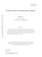
GRAVITON
Spin/
M
2
α


-4 0 4 8
2
Figure 2.1: Mass spectrum of the closed bosonic string
It shows that we have looked at the theory in an unstable vacuum. One possibility
that this is not complete nonsense could be that apart from the massterm the tachyon
potential receives higher order corrections (like e.g. a power of four term) with the
opposite sign. Then it would look rather like a Higgs field than a tachyon, and one
would expect some phase transition (tachyon condensation) to occur such that the
final theory is stable. For the moment, however, let us ignore this problem (it will not
occur in the supersymmetric theories to be studied next).
The massless particles are described by (2.1.2.22). The part symmetric in i, j and
traceless corresponds to a targetspace graviton. This is one of the most important
results in string theory. There is a graviton in the spectrum and hence string theory
can give meaning to the concept of quantum gravity. (Since Einstein gravity cannot
be quantized in a straightforward fashion there is a graviton only classically. This
corresponds to the gravitational wave solution of the Einstein equations. The particle
aspect of the graviton is missing without string theory.) The trace-part of (2.1.2.22) is
called dilaton whereas the piece antisymmetric in i, j is simply the antisymmetric ten-
sor field (commonly denoted with B). A schematic summary of the particle spectrum
of the closed bosonic string is drawn in figure 2.1.
As a consistency check one may observe that the massive excitations fit in SO(25)
representations, i.e. they form massive representations of the little group of the Lorentz
group in 26 dimensions.
As we have already mentioned, this theory contains a graviton, which is good since
it gives the prospect of quantizing gravity. On the other hand, there is the tachyon, at
best telling us that we are in the wrong vacuum. (There could be no stable vacuum
at all – for example if the tachyon had a run away potential.) Further, there are no
2. Quantization of the fundamental string 19
target space fermions in the spectrum. So, we would like to keep the graviton but to

get rid of the tachyon and add fermions. We will see that this goal can be achieved
by quantizing the supersymmetric theories.
2.1.2.2 Type II strings
In this section we are going to quantize the (1,1) worldsheet supersymmetric string.
We will follow the lines of the previous section but need to add some new ingredients.
We start with the action (2.1.1.15). The equations of motion for the bosons X
µ
are
identical to the bosonic string. So, the mode expansion of the X
µ
is not altered and
given by (2.1.2.3) and (2.1.2.4). The equations of motion for the fermions are,
∂
−
ψ
µ
+
= 0, (2.1.2.29)
∂
+
ψ
µ
−
= 0. (2.1.2.30)
Further, we need to discuss boundary conditions for the worldsheet fermions. Modulo
the equations of motion (2.1.2.29) and (2.1.2.30) the variation of the action (2.1.1.15)
with respect to the worldsheet fermions turns out to be
10
i
2π


−ψ
+µ
δψ
µ
+
+ ψ
−µ
δψ
µ
−



π
σ=0
. (2.1.2.31)
For the closed string we need to take the variation of ψ
µ
+
independent from the one of
ψ
µ
−
at the boundary (because we do not want the boundary condition to break part
of the supersymmetry (2.1.1.22) and (2.1.1.23)). Hence, the spinor components can
be either periodic or anti-periodic under shifts of σ by π. The first option gives the
Ramond (R) sector. In the R sector the general solution to (2.1.2.29) and (2.1.2.30)
can be written in terms of the following mode expansion
ψ

µ
−
=

n∈Z
d
µ
n
e
−2in(τ−σ)
, (2.1.2.32)
ψ
µ
+
=

n∈Z
˜
d
µ
n
e
−2in(τ +σ)
. (2.1.2.33)
The other option to solve the boundary condition is to take anti-periodic boundary
conditions. This is called the Neveu Schwarz (NS) sector. In the NS sector the general
solution to the equations of motion (2.1.2.29) and (2.1.2.30) reads
11
ψ
µ

−
=

r∈Z+
1
2
b
µ
r
e
−2ir(τ −σ)
, (2.1.2.34)
ψ
µ
+
=

r∈Z+
1
2
˜
b
µ
r
e
−2ir(τ+σ)
, (2.1.2.35)
10
Again we put α


=
1
2
.
11
The reality (Majorana) condition on the worldsheet spinor components provides relations analo-
gous to (2.1.2.5).
2. Quantization of the fundamental string 20
where now the sum is over half integer numbers (. . . , −
1
2
,
1
2
,
3
2
, . . .).
For the bosons the canonical commutators are as given in (2.1.2.7), (2.1.2.8).
Hence, the oscillator modes satisfy again the algebra (2.1.2.10) – (2.1.2.12). World-
sheet fermions commute with worldsheet bosons. The canonical (equal time) anti-
commutators for the fermions are

ψ
µ
+
(σ) , ψ
ν
+


σ


=

ψ
µ
−
(σ) , ψ
ν
−

σ


= πη
µν
δ

σ − σ


, (2.1.2.36)

ψ
µ
+
(σ) , ψ
ν
−


σ


= 0. (2.1.2.37)
For the Fourier modes this implies
{b
µ
r
, b
ν
s
} =

˜
b
µ
r
,
˜
b
ν
s

= η
µν
δ
r+s
(2.1.2.38)
in the NS sectors

12
, and
{d
µ
m
, d
ν
n
} =

˜
d
µ
m
,
˜
d
ν
n

= η
µν
δ
m+n
(2.1.2.39)
in the R sectors. Like the bosonic Fourier modes these can be split into creation
operators with negative Fourier index, and annihilation operators with positive Fourier
index. What about zero Fourier index? For the NS sector fermions this does not occur.
The vacuum is always taken to be an eigenstate of the bosonic zero modes where the
eigenvalues are the target space momentum of the state. (This is exactly like in the

bosonic string discussed in the previous section.) The Ramond sector zero modes
form a target space Clifford algebra (cf (2.1.2.39)). This means that the Ramond
sector states form a representation of the d dimensional Clifford algebra, i.e. they are
target space spinors. We will come back to this later. Pairing left and right movers,
there are altogether four different sectors to be discussed: NSNS, NSR, RNS, RR.
In the NSNS sector for example the left and right moving worldsheet fermions have
both anti-periodic boundary conditions. The vacuum in the NSNS sector is defined
via (2.1.2.16), (2.1.2.17) and
b
µ
r
|k =
˜
b
µ
r
|k = 0 for r > 0. (2.1.2.40)
We can build states out of this by acting with bosonic left and right moving creation
operators on it. Further, left and right moving fermionic creators from the NS sectors
can act on (2.1.2.40). We should also impose the constraints (2.1.1.24) – (2.1.1.27) on
those states. As before, we do so by going to the light cone gauge
α
+
n
= ˜α
+
n
= b
+
r

=
˜
b
+
r
= 0. (2.1.2.41)
12
We say NS sectors and not NS sector because there are two of them: a left and a right moving
one.
2. Quantization of the fundamental string 21
Then the constraints can be solved to eliminate the minus directions. The important
information is again in the zero mode of the minus direction. This reads (2.1.2.18)
2p
+
p
−
− p
i
p
i
= 8(N
NS
− a
NS
) = 8(
˜
N
NS
− a
NS

). (2.1.2.42)
The expressions for the number operators are modified due to the presence of (NS
sector) worldsheet fermions
N
NS
=
∞

n=1
α
i
−n
α
i
n
+
∞

r=
1
2
rb
i
−r
b
i
r
, (2.1.2.43)
and the analogous expression for
˜

N
NS
. Its action on states is like in the bosonic
case (see discussion below (2.1.2.20)) taking into account the appearance of fermionic
creation operators. Again, we have put a so far undetermined normal ordering constant
in (2.1.2.42) and taken normal ordered expressions for the number operators. Now,
the first excited state is
b
i
−
1
2
˜
b
j
−
1
2
|k. (2.1.2.44)
Its target space tensor structure is identical to the one of (2.1.2.22). In particular it
forms massless representations of the target space Lorentz symmetry. Thus, Lorentz
covariance implies that
a
NS
=
1
2
(2.1.2.45)
should hold.
We compute now a

NS
by first naturally assuming that a symmetrized expression
appears on the rhs of (2.1.2.42). This gives (see also (2.1.2.25))
a
NS
= −
d − 2
2
∞

n=1
n +
d −2
2
∞

r=
1
2
r. (2.1.2.46)
We use again the zeta function regularization to make sense out of (2.1.2.46). For the
second sum the following formula proves useful
∞

n=0
(n + c) = ζ (−1, c) = −
1
12

6c

2
− 6c + 1

. (2.1.2.47)
(Note, that splitting the lhs of (2.1.2.47) into ζ (−1)+c+cζ (0) gives a different (wrong)
result. This is because we understand the infinite sum as an analytic continuation of
a finite one:

(n + a)
−s
with real part of s greater than one. For generic s the above