Oracle SQL Tuning with Oracle SQLTXPLAIN doc
Bạn đang xem bản rút gọn của tài liệu. Xem và tải ngay bản đầy đủ của tài liệu tại đây (10.33 MB, 333 trang )
www.it-ebooks.info
For your convenience Apress has placed some of the front
matter material after the index. Please use the Bookmarks
and Contents at a Glance links to access them.
www.it-ebooks.info
v
Contents at a Glance
About the Author ���������������������������������������������������������������������������������������������������������������� xv
About the Technical Reviewer ������������������������������������������������������������������������������������������xvii
Acknowledgments ������������������������������������������������������������������������������������������������������������� xix
Foreword ��������������������������������������������������������������������������������������������������������������������������� xxi
Introduction ���������������������������������������������������������������������������������������������������������������������� xxv
Chapter 1: Introduction to SQLTXPLAIN ■ �����������������������������������������������������������������������������1
Chapter 2: The Cost-Based Optimizer Environment ■ ��������������������������������������������������������17
Chapter 3: How Object Statistics Can Make Your Execution Plan Wrong ■ ������������������������39
Chapter 4: How Skewness Can Make Your Execution Times Variable ■ �����������������������������53
Chapter 5: Troubleshooting Query Transformations ■ ��������������������������������������������������������71
Chapter 6: Forcing Execution Plans Through Profiles ■ �����������������������������������������������������93
Chapter 7: Adaptive Cursor Sharing ■ ������������������������������������������������������������������������������111
Chapter 8: Dynamic Sampling and Cardinality Feedback ■ ���������������������������������������������129
Chapter 9: Using SQLTXPLAIN with Data Guard Physical Standby Databases ■ ���������������147
Chapter 10: Comparing Execution Plans ■ �����������������������������������������������������������������������163
Chapter 11: Building Good Test Cases ■ ���������������������������������������������������������������������������177
Chapter 12: Using XPLORE to Investigate Unexpected Plan Changes ■ ����������������������������205
Chapter 13: Trace Files, TRCANLZR and Modifying SQLT behavior ■ ��������������������������������231
www.it-ebooks.info
■ Contents at a GlanCe
vi
Chapter 14: Running a Health Check ■ �����������������������������������������������������������������������������255
Chapter 15: The Final Word ■ �������������������������������������������������������������������������������������������281
Appendix A: Installing SQLTXPLAIN ■ �������������������������������������������������������������������������������285
Appendix B: The CBO Parameters (11�2�0�1) ■ �����������������������������������������������������������������295
Appendix C: Tool Configuration Parameters ■ ������������������������������������������������������������������307
Index ���������������������������������������������������������������������������������������������������������������������������������311
www.it-ebooks.info
xxv
Introduction
is book is intended as a practical guide to an invaluable tool called SQLTXPLAIN, commonly known simply as
SQLT. You may never have heard of it, but if you have anything to do with Oracle tuning, SQLT is one of the most
useful tools you’ll nd. Best of all, it’s freely available from Oracle. All you need to do is learn how to use it.
How This Book Came to Be Written
I’ve been a DBA for over twenty years. In that time, I dealt with many, many tuning problems yet it was only when I
began to work for Oracle that I learned about SQLT. As a part of the tuning team at Oracle Support I used SQLT every
day to solve customers’ most complex tuning problems. I soon realized that my experience was not unique. Outside
Oracle, few DBAs knew that SQLT existed. An even smaller number knew how to use it. Hence the need for this book.
Don’t Buy This Book
If you’re looking for a text on abstract tuning theory or on how to tune “raw” SQL. is book is about how to use SQLT
to do Oracle SQL tuning. e approach used is entirely practical and uses numerous examples to show the SQLT tool
in action.
Do Buy This Book
If you’re a developer or a DBA and are involved with Oracle SQL tuning problems. No matter how complex your
system or how many layers of technology there are between you and your data, getting your query to run eciently
is where the rubber meets the road. Whether you’re a junior DBA, just starting your career, or an old hand who’s seen
it all before, this book is designed to show you something completely practical that will be useful in your day-to-day
work.
An understanding of SQLT will radically improve your ability to solve tuning problems and will also give you an
eective checklist to use against new code and old.
Tuning problems are among the most complex technical problems around. SQLTXPLAIN is a fantastic tool that
will help you solve them. Prepare to be smitten.
www.it-ebooks.info
1
Chapter 1
Introduction to SQLTXPLAIN
Welcome to the world of fast Oracle SQL tuning with SQLTXPLAIN, or SQLT as it is typically called. Never heard of
SQLT? You’re not alone. I’d never heard of it before I joined ORACLE, and I had been a DBA for more years than I care
to mention. That’s why I’m writing this book. SQLT is a fantastic tool because it helps you diagnose tuning problems
quickly. What do I mean by that? I mean that in half a day, maximum, you can go from a slow SQL to having an
understanding of why SQL is malfunctioning, and finally, to knowing how to fix the SQL.
Will SQLT fix your SQL? No. Fixing the SQL takes longer. Some tables are so large that it can take days to gather
statistics. It may take a long time to set up the test environment and roll the fix to production. The important point is
that in half a day working with SQLT will give you an explanation. You’ll know why the SQL was slow, or you’ll be able
to explain why it can’t go any faster.
You need to know about SQLT because it will make your life easier. But let me back up a little and tell you more
about what SQLT is, how it came into existence, why you probably haven’t heard of it, and why you should use it for
your Oracle SQL tuning.
What Is SQLT?
SQLT is a set of packages and scripts that produces HTML-formatted reports, some SQL scripts and some text files.
The entire collection of information is packaged in a zip file and often sent to Oracle Support, but you can look at
these files yourself. There are just over a dozen packages and procedures (called “methods”) in SQLT. These packages
and procedures collect different information based on your circumstances. We’ll talk about the packages suitable for a
number of situations later.
What’s the Story of SQLT?
They say that necessity is the mother of invention, and that was certainly the case with SQLT. Oracle support engineers
handle a huge number of tuning problems on a daily basis; problem is, the old methods of linear analysis are just too
slow. You need to see the big picture fast so you can zoom in on the detail and tell the customer what’s wrong. As
a result, Carlos Sierra, a support engineer at the time (now a member of the Oracle Center of Expertise—a team of
experts within Oracle) created SQLT. The routines evolved over many visits to customer sites to a point where they can
gather all the information required quickly and effectively. He then provided easy-to-use procedures for reporting on
those problems.
Carlos Sierra, the genius of SQLT, now spends much of his time improving SQLT code and adapting the SQLT
code to new versions of the RDBMS. He also assists Oracle Tuning Performance engineers with SQL tuning through
the medium of SQLT.
www.it-ebooks.info
Chapter 1 ■ IntroduCtIon to SQLtXpLaIn
2
Why Haven’t You Heard of SQLT?
If it’s so useful, why haven’t you heard about SQLT? Oracle has tried to publicize SQLT to the DBA community, but still
I get support calls and talk to DBAs who have never heard of SQLT—or if they have, they’ve never used it. This amazing
tool is free to supported customers, so there’s no cost involved. DBAs need to look at problematic SQL often, and
SQLT is hands down the fastest way to fix a problem. The learning curve may be high, but it’s nowhere near as high as
the alternatives: interpreting raw 10046 trace files or 10053 trace files. Looking through tables of statistics to find the
needle in the haystack, guessing about what might fix the problem and trying it out? No thanks. SQLT is like a cruise
missile that travels across the world right to its target.
Perhaps DBAs are too busy to learn a tool, which is not even mentioned in the release notes for Oracle. It’s not
in the documentation set, it’s not officially part of the product set either. It’s just a tool, written by a talented support
engineer, and it happens to be better than any other tool out there. Let me repeat. It’s free.
It’s also possible that some DBAs are so busy focusing on the obscure minutiae of tuning that they forget the real
world of fixing SQL. Why talk about a package that’s easy to use when you could be talking about esoteric hidden
parameters for situations you’ll never come across? SQLT is a very practical tool.
Whatever the reason, if you haven’t used SQLT before, my mission in this book is to get you up and running as
fast and with as little effort from you as possible. I promise you installing and using SQLT is easy. Just a few simple
concepts, and you’ll be ready to go in 30 minutes.
How Did I Learn About SQLT?
Like the rest of the DBA world (I’ve been a DBA for many years), I hadn’t heard of SQLT until I joined Oracle. It was a
revelation to me. Here was this tool that’s existed for years, which was exactly what I needed many times in the past,
although I’d never used it. Of course I had read many books on tuning in years past: for example, Cary Millsaps’s
classic Optimizing Oracle Performance, and of course Cost-Based Oracle Fundamentals by Jonathan Lewis.
The training course (which was two weeks in total) was so intense that it was described by at least two engineers
as trying to drink water from a fire hydrant. Fear not! This book will make the job of learning to use SQLT much easier.
Now that I’ve used SQLT extensively in day-to-day tuning problems, I can’t imagine managing without it. I want
you to have the same ability. It won’t take long. Stick with me until the end of the book, understand the examples, and
then try and relate them to your own situation. You’ll need a few basic concepts (which I’ll cover later), and then you’ll
be ready to tackle your own tuning problems. Remember to use SQLT regularly even when you don’t have a problem;
this way you can learn to move around the main HTML file quickly to find what you need. Run a SQLT report against
SQL that isn’t a problem. You’ll learn a lot. Stick with me on this amazing journey.
Getting Started with SQLT
Getting started with SQLT couldn’t be easier. I’ve broken the process down into three easy steps.
1. Downloading SQLT
2. Installing SQLT
3. Running your first SQLT report
SQLT will work on many different platforms. Many of my examples will be based on Microsoft Windows, but
Linux or Unix is just as easy to use, and there are almost no differences in the use of SQLT between the platforms. If
there are, I’ll make a note in the text.
www.it-ebooks.info
Chapter 1 ■ IntroduCtIon to SQLtXpLaIn
3
How Do You Get a Copy of SQLT?
How do you download SQLT? It’s simple and easy. I just did it to time myself. It took two minutes. Here are the steps to
get the SQLT packages ready to go on your target machine:
1. Find a web browser and log in to My Oracle Support ()
2. Go to the knowledge section and type “SQLT” in the search box. Note 215187.1 entitled
“SQLT (SQLTXPLAIN) – Tool that helps to diagnose a SQL statement performing poorly
[ID 215187.1]” should be at the top of the list.
3. Scroll to the bottom of the note and choose the version of SQLT suitable for your
environment. There are currently versions suitable from 9i to 11 g.
4. Download the zip file (the version I downloaded was 2Mbytes).
5. Unzip the zip file.
You now have the SQLT programs available to you for installation onto any suitable database. You can download
the zip file to a PC and then copy it to a server if needed.
How Do You Install SQLT?
So without further ado, let’s install SQLT so we can do some tuning:
1. Download the SQLT zip file appropriate for your environment (see steps above).
2. Unzip the zip file to a suitable location.
3. Navigate to your “install” directory under the unzipped area (in my case it is C:\Document
and Settings\Stelios\Desktop\SQLT\sqlt\install, your locations will be different).
4. Connect as sys, e.g., sqlplus / as sysdba
5. Make sure your database is running
6. Run the sqcreate.sql script.
7. Select the default for the first option. (We’ll cover more details of the installation in
Appendix A.)
8. Enter and confirm the password for SQLTXPLAIN (the owner of the SQLT packages).
9. Select the tablespace where the SQLTXPLAIN will keep its packages and data
(in my case, USERS).
10. Select the temporary tablespace for the SQLTXPLAIN user (in my case, TEMP).
11. Then enter the username of the user in the database who will use SQLT packages to fix
tuning problems. Typically this is the schema that runs the problematic SQL (in my case
this is STELIOS).
12. Then enter “T”, “D” or “N.” This reflects your license level for the tuning and diagnostics
packs. Most sites have both so you would enter “T”, (this is also the default). My test system
is on my PC (an evaluation platform with no production capability) so I would also enter
“T”. If you have the diagnostics pack, only enter “D”; and if you do not have these licenses,
enter “N”.
The last message you see is “SQCREATE completed. Installation completed successfully.”
www.it-ebooks.info
Chapter 1 ■ IntroduCtIon to SQLtXpLaIn
4
Running Your First SQLT Report
Now that SQLT is installed, it is ready to be used. Remember that installing the package is done as sys and that
running the reports is done as the target user. Please also bear in mind that although I have used many examples from
standard schemas available from the Oracle installation files, your platform and exact version of Oracle may well be
different, so please don’t expect your results to be exactly the same as mine. However, your results will be similar to
mine, and the results you see in your environment should still make sense.
1. Now exit SQL and change your directory to \SQLT\run. In my case this is C:\Documents
and Settings\Stelios\Desktop\SQLT\sqlt\run. From here log in to SQLPLUS as the
target user.
2. Then enter the following SQL (this is going to be the statement we will tune):
SQL > select count(*) from dba_objects;
3. Then get the SQL_ID value from the following SQL
SQL > select sql_id from v$sqlarea where sql_text like 'select count(*) from
dba_objects%';
In my case the SQL_ID was g4pkmrqrgxg3b.
4. Now we execute our first SQLT tool sqltxtract from the target schema (in this case
STELIOS) with the following command:
SQL > @sqltxtract g4pkmrqrgxg3b
5. Enter the password for SQLTXPLAIN (which you entered during the installation). The last
message you will see if all goes well is “SQLTXTRACT completed”.
6. Now create a zip directory under the run directory and copy the zip file created into the
zip directory. Unzip it.
7. Finally from your favorite browser navigate to and open the file named
sqlt_s <nnnnn> _main.html. The symbols “nnnnn” represent numbers created to make all
SQLT reports unique on your machine. In my case the file is called sqlt_s89906_main.html
Congratulations! You have your first SQLT XTRACT report to look at.
When to Use SQLTXTRACT and When to Use SQLTXECUTE
SQLT XTRACT is the easiest report to create because it does not require the execution of the SQL at the time of the
report generation. The report can be collected after the statement has been executed. SQLTXECUTE, on the other
hand, executes the SQL statement and thus has better run-time information and access to the actual rows returned.
This means it can assess the accuracy of the estimated cardinality of the steps in the execution plan (see “Cardinality
and Selectivity” later in this chapter). SQLTXECUTE will get you more information, but it is not always possible to use
this method, perhaps because you are in a production environment or perhaps the SQL statement is currently taking
three days to run, which is why you are investigating this in the first place. We will look at both SQLTXECUTE and
SQLTXTRACT report (and other SQLT options also). For now we will concentrate on one simple SQLTXTRACT report
on a very simple SQL statement. So let’s dive in.
www.it-ebooks.info
Chapter 1 ■ IntroduCtIon to SQLtXpLaIn
5
Your First SQLT Report
Before we get too carried away with all the details of using the SQLT main report, just look at Figure 1-1. It’s the
beginning of a whole new SQLT tuning world. Are you excited? You should be. This header page is just the beginning.
From here we will look at some basic navigation, just so you get an idea of what is available and how SQLT works, in
terms of its navigation. Then we’ll look at what SQLT is actually reporting about the SQL.
Figure 1-1. The top part of the SQLT report shows the links to many areas
Some Simple Navigation
Let’s start with the basics. Each hyperlinked section has a Go to Top hyperlink to get you back to the top. There’s a lot
of information in the various sections, and you can get lost. Other related hyperlinks will be grouped together above
the Go to Top hyperlink. For example, if I clicked on Indexes (the last link under the Tables heading), I would see the
page shown in Figure 1-2.
www.it-ebooks.info
Chapter 1 ■ IntroduCtIon to SQLtXpLaIn
6
Before we get lost in the SQLT report let’s again look at the header page (Figure 1-1). The main sections cover all
sorts of aspects of the system.
CBO environment
Cursor sharing
Adaptive cursor sharing
SQL Tuning Advisor (STA) report
Execution plan(s) (there will be more than one plan if the plan changed)
SQL*Profiles
Outlines
Execution statistics
Table metadata
Index metadata
Column definitions
Foreign keys
Take a minute and browse through the report.
Figure 1-2. The Indexes section of the report
Chapter 1 ■ IntroduCtIon to SQLtXpLaIn
7
Did you notice the hyperlinks on some of the data within the tables? SQLT collected all the information it could
find and cross-referenced it all.
So for example, continuing as before from the main report at the top (Figure 1-1)
1. Click on Indexes, the last heading under Tables.
2. Under the Indexes column of the Indexes heading, the numbers are hyperlinked (see
Figure 1-2). I clicked on 2 of the USERS$ record.
Now you can see the details of the columns in that table (see Figure 1-3). As an example
here we see that the index I_USER2 was used in the execution of my query (the In Plan
column value is set to TRUE).
Figure 1-3. An Index’s detailed information about statistics
3. Now, in the Index Meta column (far right in Figure 1-3), click on the Meta hyperlink for the
I_USER2 index to display the index metadata shown in Figure 1-4.
Chapter 1 ■ IntroduCtIon to SQLtXpLaIn
8
Here we see the statement we would need to create this index. Do you have a script to do that? Well SQLT can
get it better and faster. So now that you’ve seen a SQLT report, how do you approach a problem? You’ve opened the
report, and you have one second to decide. Where do you go?
Well, that all depends.
How to Approach a SQLT Report
As with any methodology, different approaches are considered for different circumstances. Once you’ve decided there
is something wrong with your SQL, you could use a SQLT report. Once you have the SQLT report, you are presented
with a header page, which can take you to many different places (no one reads a SQLT report from start to finish in
order). So where do you go from the main page?
If you’re absolutely convinced that the execution plan is wrong, you might go straight to “Execution Plans” and
look at the history of the execution plans. We’ll deal with looking at those in detail later.
Suppose you think there is a general slowdown on the system. Then you might want to look at the “Observations”
section of the report.
Maybe something happened to your statistics, so you’ll certainly need to look at the “Statistics” section of the
report under “Tables.”
All of the sections I’ve mentioned above are sections you will probably refer to for every problem. The idea is to
build up a picture of your SQL statement, understand the statistics related to the query, understand the cost-based
optimizer (CBO) environment and try and get into its “head.” Why did it do what it did? Why does it not relate to
what you think it ought to do? The SQLT report is the explanation from the optimizer telling you why it decided to
do what it did. Barring the odd bug, the CBO usually has a good reason for doing what it did. Your job is to set up the
environment so that the CBO agrees with your worldview and run the SQL faster!
Figure 1-4. Metadata about an index can be seen from the “Meta” hyperlink
Chapter 1 ■ IntroduCtIon to SQLtXpLaIn
9
Cardinality and Selectivity
My objective throughout this book, apart from making you a super SQL tuner, is to avoid as much jargon as possible
and explain tuning concepts as simply as possible. After all we’re DBAs, not astrophysicists or rocket scientists.
So before explaining some of these terms it is important to understand why these concepts are key to the CBO
operation and to your understanding of the SQL running on your system. Let’s first look at cardinality. It is defined as
the number of rows expected to be returned for a particular column if a predicate selects it. If there are no statistics for
the table, then the number is pretty much based on heuristics about the number of rows, the minimum and maximum
values, and the number of nulls. If you collect statistics then these statistics help to inform the guess, but it’s still a
guess. If you look at every single row of a table (collecting 100 percent statistics), it might still be a guess because the
data might have changed, or the data may be skewed (we’ll cover skewness later). That dry definition doesn’t really
relate to real life, so let’s look at an example. Click on the “Execution Plans” hyperlink at the top of the SQLT report to
display an execution plan like the one shown in Figure 1-5.
In the “Execution Plan” section, you’ll see the “Estim Card” column. In my example, look at the TABLE ACCESS
FULL OBJ$ step. Under the “Estim Card” column the value is 73,572. Remember cardinality is the number of rows
returned from a step in an execution plan. The CBO (based on the table’s statistics) will have an estimate for the
cardinality. The “Estim Card” column then shows what the CBO expected to get from the step in the query. The 73,572
shows that the CBO expected to get 73,572 records from this step, but in fact got 73,235. So how good was the CBO’s
estimate for the cardinality (the number of rows returned for a step in an execution plan)? In our simple example we
can do a very simple direct comparison by executing the query show below.
Figure 1-5. An execution plan in the “Execution Plan” section
Chapter 1 ■ IntroduCtIon to SQLtXpLaIn
10
SQL> select count(*) from dba_objects;
COUNT(*)
73235
SQL>
So cardinality is the actual number of rows that will be returned, but of course the optimizer can’t know the
answers in advance. It has to guess. This guess can be good or bad, based on statistics and skewness. Of course,
histograms can help here.
For an example of selectivity, let’s look at the page (see Figure 1-6) we get by selecting Columns from the Tables
options on the main page (refer to Figure 1-1).
Look at the “SYS.IND$ - Table Column” section. From the “Table Columns” page, if we click on the “34” under
the “Column Stats” column, we will see the column statistics for the SYS.IND$ index. Figure 1-7 shows a subset of the
page from the “High Value” column to the “Equality Predicate Cardinality” column. Look at the “Equality Predicate
Selectivity” and “Equality Predicate Cardinality” columns (the last two columns). Look at the values in the first row
for OBJ#.
Figure 1-6. The “Table Column” section of the SQLT report
Chapter 1 ■ IntroduCtIon to SQLtXpLaIn
11
Selectivity is 0.000209, and cardinality is 1.
This translates to “I expect to get 1 row back for this equality predicate, which is equivalent to a 0.000209 chance
(1 is certainty 0 is impossible) or in percentage terms I’ll get 0.0209 percent of the entire table if I get the matching
rows back.”
Notice that as the cardinality increases the selectivity also increases. The selectivity only varies between 0 and 1
(or if you prefer 0 percent and 100 percent) and cardinality should only vary between 0 and the total number of rows
in the table (excluding nulls). I say should because these values are based on statistics. What would happen if you
gathered statistics on a partition (say it had 10 million rows) and then you truncate that partition, but don’t tell the
optimizer (i.e., you don’t gather new statistics, or clear the old ones). If you ask the CBO to develop an execution plan
in this case it might expect to get 10 million rows from a predicate against that partition. It might “think” that a full
table scan would be a good plan. It might try to do the wrong thing because it had poor information.
To summarize, cardinality is the count of expected rows, and selectivity is the same thing but on a 0–1 scale. So
why is all this important to the CBO and to the development of good execution plans? The short answer is that the
CBO is working hard for you to develop the quickest and simplest way to get your results. If the CBO has some idea
about how many rows will be returned for steps in the execution plan, then it can try variations in the execution plan
and choose the plan with the least work and the fastest results. This leads into the concept of “cost,” which we will
cover in the next section.
What Is Cost?
Now that we have cardinality for an object we can work with other information derived from the system to calculate a
cost for any operation. Other information from the system includes the following:
Speed of the disks
Speed of the CPU
Number of CPUs
Database block size
These metrics can be easily extracted from the system and are shown in the SQLT report also (under the
“Environment” section). The amount of I/O and CPU resource used on the system for any particular step can now
be calculated and thus used to derive a definite cost. This is the key concept for all tuning. The optimizer is always
trying to reduce the cost for an operation. I won’t go into details about how these costs are calculated because the
exact values are not important. All you need to know is this: higher is worse, and worse can be based on higher cardinality
(possibly based on out-of-date statistics), and if your disk I/O speeds are wrong (perhaps optimistically low) then full
table scans might be favored when indexes are available. Cost can also be directly translated into elapsed time (on a quiet
system), but that probably isn’t what you need most of the time because you’re almost always trying to get an execution
time to be reduced, i.e., lower cost. As we’ll see in the next section, you can get that information from SQLT. SQLT will also
produce a 10053 trace file in some cases, so you can look at the details of how the cost calculations are made.
Figure 1-7. Selectivity is found in the “Equality Predicate Selectivity” column
Chapter 1 ■ IntroduCtIon to SQLtXpLaIn
12
Reading the Execution Plan Section
We saw the execution plan section previously. It looks interesting, and it has a wobbly left edge and lots of hyperlinks.
What does it all mean? This is a fairly simple execution plan, as it doesn’t go on for pages and pages (like SIEBEL or
PeopleSoft execution plans).
There are a number of simple steps to reading an execution plan. I’m sure there’s more than one way of reading
an execution plan, but this is the way I approach the problem. Bear in mind in these examples that if you are familiar
with the pieces of SQL being examined, you may go directly to the section you think is wrong; but in general if you are
seeing the execution plan for the first time, you will start by looking at a few key costs.
The first and most important cost is the overall cost of the entire query. This is always shown as “ID 0” and is
always the first row in the execution plan. In our example shown in Figure 1-5, this is a cost of 256. So to get the cost
for the entire query just look at the first row. This is also the last step to be executed (“Exec Ord” is 18). The execution
order is not top to bottom, the Oracle engine will carry out the steps in the order shown by the value in the “Exec Ord”
column. So if we followed the execution through, the Oracle engine would do the execution in this order:
1. INDEX FULL SCAN I_USER2
2. INDEX FULL SCAN I_USER2
3. TABLE ACCESS FULL OBJ$
4. HASH JOIN
5. HASH JOIN
6. INDEX UNIQUE SCAN I_IND1
7. TABLE ACCESS BY INDEX ROWID IND$
8. INDEX FULL SCAN I_USERS2
9. INDEX RANGE SCAN I_OBJ4
10. NESTED LOOP
11. FILTER
12. INDEX FULL SCAN I_LINK1
13. INDEX RANGE SCAN I_USERS2
14. NESTED LOOPS
15. UNION-ALL
16. VIEW DBA_OBJECTS
17. SORT AGGREGATE
18. SELECT STATEMENT
However, nobody ever represents the plan of a SQL statement like this. What is important to realize is that the
wobbly left edge gives information about how the steps are carried out. The less-indented operations indicate outer
operations that are being carried out on inner (more indented) operations. So for example steps 2, 3, and 4 would be
read as “An index full scan is carried out using I_USERS2, then a full table scan of OBJ$ and the results of these are HASH
JOINED to produce a result set.” Each operation produces results for a less-indented section until the final result is
presented to the SELECT (ID = 0).
Chapter 1 ■ IntroduCtIon to SQLtXpLaIn
13
The “Operation” column is also marked with “+” and “–” to indicate sections of equal indentation. This is helpful
in lining up operations to see which result sets an operation is working on. So, for example, it is important to realize
that the HASH JOIN at step 5 is using results from steps 1, 4, 2, and 3. We’ll see more complex examples of these later.
It is also important to realize that the costs shown are aggregate costs for each operation as well. So the cost shown on
the first line is the cost for the entire operation, and we can also see that most of the cost of the entire operation came
from step 3. (SQLT helpfully shows the highest cost operation in red). So let’s look at step 1 (as shown in Figure 1-5) in
more detail. In our simple case this is
"INDEX FULL SCAN I_USER2"
Let’s translate the full line into English: “First get me a full index scan of index I_USERS2. I estimate 93 rows will be
returned which, based on your current system statistics (Single block read time and multi-block read times and CPU
speed), will be a cost of 1.”
The second and third steps are another INDEX FULL SCAN and a TABLE ACCESS FULL of OBJ$. This third step
has a cost of 251. The total cost of the entire SQL statement is 256 (top row). So if were looking to tune this statement
we know that the benefit must come from this third step (it is a cost of 251 out of a total cost of 256). Now place your
cursor over the word “TABLE” on step 3 (see Figure 1-8).
Figure 1-8. More details can be obtained by ‘hovering’ over links
Chapter 1 ■ IntroduCtIon to SQLtXpLaIn
14
Notice how information is displayed about the object.
Object#: 18
Owner: SYS
Qblock: SEL$1FF6F973
Alias: O@SEL$4
Current Table Statistics:
Analyzed: 08-JUN-12 22:01:24
TblRows: 73575
Blocks: 905
Sample 73575
Just by hovering your mouse over the object you get its owner, the query block name, when it was last analyzed,
and how big the object is.
Now let’s look at the “Go To” column. Notice the “+” under that column? Click on the one for step 3, and you’ll get
a result like the one in Figure 1-9.
Figure 1-9. More hyperlinks can be revealed by expanding sections on the execution plan
Chapter 1 ■ IntroduCtIon to SQLtXpLaIn
15
So right from the execution plan you can go to the “Col Statistics” or the “Stats Versions” or many other things.
You decide where you want to go next, based on what you’ve understood so far and on what you think is wrong
with your execution plan. Now close that expanded area and click on the “+” under the “More” column for step 3
(see Figure 1-10)
Figure 1-10. Here we see an expansion under the “More” heading
Now we see the filter predicates and the projections. These can help you understand which line in the execution
plan the optimizer is considering predicates for and which values are in play for filters.
Just above the first execution plan is a section called “Execution Plans.” This lists all the different execution plans
the Oracle engine has seen for this SQL. Because execution plans can be stored in multiple places in the system, you
could well have multiple entries in the “Execution Plans” section of the report. Its source will be noted (under the
“Source” column). Here is a list of sources I’ve come across:
GV$SQL_PLAN
GV$SQLAREA_PLAN_HASH
PLAN_TABLE
DBA_SQLTUNE_PLANS
DBA_HIST_SQL_PLAN
SQLT will look for plans in as many places as possible so that it can you give you a full range of options. When
SQLT gathers this information, it will look at the cost associated with each of these plans and label them with “W”
in red (worst) and “B” in green (best). In my simple test case, the “Best” and “Worst” are the same, as there is only
one execution plan in play. However you’ll notice there are three records: one came from mining the memory
GV$SQL_PLAN, one came from PLAN_TABLE (i.e., an EXPLAIN PLAN) and one came from DBA_SQLTUNE_PLANS,
(SQL Tuning Analyzer) whose source is DBA_SQLTUNE_PLANS.
When you have many records here, perhaps a long history, you can go back and see which plans were best and
try to see why they changed. Noting the timing of a change can sometimes be crucial, as it can help you zoom in on
the change that made things worse.
4
Chapter 1 ■ IntroduCtIon to SQLtXpLaIn
16
Before we launch into even more detailed use of the “Execution Plans” section, we’ll need more complex
examples.
Join Methods
This book is focused on very practical tuning with SQLT. I try to avoid unnecessary concepts and tuning minutiae.
For this reason I will not cover every join method available or every DBA table that might have some interesting
information about performance or every hint. These are well documented in multiple sources, not least of which
is the Oracle Performance guide (which I recommend you read). However, we need to cover some basic concepts
to ensure we get the maximum benefit from using SQLT. So, for example, here are some simple joins. As its name
implies, a join is a way of “joining” two data sets together: one might contain a person’s name and age and another
table might contain the person’s name and income level. In which case you could “join” these tables to get the names
of people of a particular age and income level. As the name of the operation implies, there must be something to join
the two data sets together: in our case, it’s the person’s name. So what are some simple joins? (i.e., ones we’ll see in
out SQLT reports).
HASH JOINS (HJ) – The smaller table is hashed and placed into memory. The larger table is
then scanned for rows that match the hash value in memory. If the larger and smaller tables
are the wrong way around this is inefficient. If the tables are not large, this is inefficient. If
the smaller table does not fit in memory, then this is more than inefficient: it’s really bad!
NESTED LOOP (NL) – Nested Loop joins are better if the tables are smaller. Notice how in
the execution plan examples above there is a HASH JOIN and a NESTED LOOP. Why was
each chosen for the task? The details of each join method and its associated cost can be
determined from the 10053 trace file. It is a common practice to promote the indexes and
NL by adjusting the optimizer parameters Optimizer_index_cost_adj and optimizer_
index_caching parameters. This is not generally a winning strategy. These parameters
should be set to the defaults of 100 and 0. Work on getting the object and system statistics
right first.
CARTESIAN JOINS – Usually bad. Every row of the first table is used as a key to access every
row of the second table. If you have a very few number of rows in the joining tables this join
is OK. In most production environments, if you see this occurring then something is wrong,
usually statistics.
SORT MERGE JOINS (SMJ) – Generally joined in memory if memory allows. If the
cardinality is high then you would expect to see SMJs and HJs.
Summary
In this chapter we covered the basics of using SQLTXTRACT. This is a simple method of SQLT that does not execute
the SQL statement in question. It extracts the information required from all possible sources and presents this in
a report.
In this chapter we looked at a simple download and install of SQLT. You’ve seen that installing SQLT on a local
database can take very little time, and its use is very simple. The report produced was easy to unzip and can be
used to investigate the SQL performance. In this first example we briefly mentioned cardinality and selectivity and
how these affect the cost-based optimizer’s plans. Now let’s investigate more of SQLT’s features and look at more
complex examples.
17
Chapter 2
The Cost-Based Optimizer
Environment
When I’m solving tricky tuning problems, I’m often reminded of the story of the alien who came to earth to try
his hand at driving. He’d read all about it and knew the physics involved in the engine. It sounded like fun. He sat
down in the driver’s seat and turned the ignition; the engine ticked over nicely, and the electrics were on. He put his
seatbelt on and tentatively pressed the accelerator pedal. Nothing happened. Ah! Maybe the handbrake was on.
He released the handbrake and pressed the accelerator again. Nothing happened. Later, standing back from the car
and wondering why he couldn’t get it to go anywhere, he wondered why the roof was in contact with the road.
My rather strange analogy is trying to help point out that before you can tune something, you need to know
what it should look like in broad terms. Is 200ms reasonable for a single block read time? Should system statistics be
collected over a period of 1 minute? Should we be using hash joins for large table joins? There are 1,001 things that to
the practiced eye look wrong, but to the optimizer it’s just the truth.
Just like the alien, the Cost Based Optimizer (CBO) is working out how to get the best performance from your
system. It knows some basic rules and guestimates (heuristics) but doesn’t know about your particular system or data.
You have to tell it about what you have. You have to tell the alien that the black round rubbery things need to be in
contact with the road. If you ‘lie’ to the optimizer, then it could get the execution plan wrong, and by wrong I mean the
plan will perform badly. There are rare cases where heuristics are used inappropriately or there are bugs in the code
that lead the CBO to take shortcuts (Query transformations) that are inappropriate and give the wrong results. Apart
from these, the optimizer generally delivers poor performance because it has poor information to start with. Give it
good information, and you’ll generally get good performance.
So how do you tell if the “environment” is right for your system? In this chapter we’ll look at a number of aspects
of this environment. We’ll start with (often neglected) system statistics and then look at the database parameters
that affect the CBO. We’ll briefly touch on Siebel environments and the have a brief look at histograms (these are
covered in more detail in the next chapter). Finally, we’ll look at both overestimates and underestimates (one of
SQLT’s best features is highlighting these), and then we’ll dive into a real life example, where you can play detective
and look at examples to hone your tuning skills (no peeking at the answer). Without further ado let’s start with
system statistics.
System Statistics
System statistics are an often-neglected part of the cost-based optimizer environment. If no system statistics have
been collected for a system then the SQLT section “Current System Statistics” will show nothing for a number of
important parameters for the system. An example is shown in Figure 2-3. It will guess these values. But why should
you care if these values are not supplied to the optimizer? Without these values the optimizer will apply its best guess
for scaling the timings of a number of crucial operations. This will result in inappropriate indexes being used when a
full table scan would do or vice versa. These settings are so important that in some dynamic environments where the
CHAPTER 2 ■ THE COST-BASED OPTIMIZER ENVIRONMENT
18
workload is changing, for example from the daytime OLTP to a nighttime DW (Data Warehouse) environment, that
different sets of system statistics should be loaded. In this section we’ll look at why these settings affect the optimizer,
how and when they should be collected, and what to look for in a SQLT report.
Figure 2-1. The top section of the SQLT report
Let’s remind ourselves what the first part of the HTML report looks like (see Figure 2-1). Remember this is one
huge HTML page with many sections.
From the main screen, in the Global section, select “CBO System Statistics”. This brings you to the section where
you will see a heading “CBO System Statistics” (See Figure 2-2).
Figure 2-2. The “CBO System Statistics” section
CHAPTER 2 ■ THE COST-BASED OPTIMIZER ENVIRONMENT
19
Now click on “Info System Statistics.” Figure 2-3 shows what you will see.
Figure 2-3. The “Info System Statistics” section
The “Info System Statistics” section shows many pieces of important information about your environment. This
screenshot also shows the “Current System Statistics” and the top of the “Basis and Synthesized Values” section.
Notice, when the System Statistics collection was started. It was begun on 23
rd
of July 2007 (quite a while ago).
Has the workload changed much since then? Has any new piece of equipment been added? New SAN drives? Faster
disks? All of these could affect the performance characteristics of the system. You could even have a system that needs
a different set of system statistics for different times of the day.
Notice anything else strange about the system statistics? The start and end times are almost identical. The start
and end time should be scheduled to collect information about the system characteristics at the start and end times
of the representative workload. These values mean that they where set at database creation time and never changed.
Look at the “Basis and Synthesized Values” sections shown in Figure 2-4.
CHAPTER 2 ■ THE COST-BASED OPTIMIZER ENVIRONMENT
20
The estimated SREADTIM (single block read time in ms.) and MREADTIM (multi-block read time in ms) are
12ms and 58ms, whereas the actual values (just below) are 3.4ms and 15ms. Are these good values? It can be hard
to tell because modern SAN systems can deliver blistering I/O read rates. For traditional non-SAN systems you would
expect multi-block read times to be higher than single block read times and the normally around 9ms and 22ms.
In this case they are in a reasonable range. The Single block read time is less than the multi-block read time
(you would expect that, right?).
Now look in Figure 2-5 at a screen shot from a different system.
Figure 2-4. From the “Basis and Synthesized Values” section just under “Info System Statistics” section
Figure 2-5. Basis and synthezed values section under Info System Statistics