Báo cáo " WATER VAPOR FEEDBACK AND GLOBAL WARMING " pot

P1: FXZ
October 16, 2000 13:0 Annual Reviews AR118-13
Annu. Rev. Energy Environ. 2000. 25:441–75
WATER VAPOR FEEDBACK AND
GLOBAL WARMING
1
Isaac M. Held and Brian J. Soden
Geophysical Fluid Dynamics Laboratory/National Oceanic and Atmospheric
Administration, Princeton, New Jersey 08542
Key Words climate change, climate modeling, radiation
■ Abstract Watervaporisthedominantgreenhouse gas, themostimportant gaseous
sourceof infraredopacity in theatmosphere. Asthe concentrationsof other greenhouse
gases, particularly carbon dioxide, increase because of human activity, it is centrally
important topredict how the watervapordistributionwill be affected. Tothe extentthat
water vapor concentrations increasein a warmer world, the climatic effects of the other
greenhouse gases will be amplified. Models of the Earth’s climate indicate that this
is an important positive feedback that increases the sensitivity of surface temperatures
to carbon dioxide by nearly a factor of two when considered in isolation from other
feedbacks, andpossibly byas muchas afactor of three or more when interactions with
other feedbacks are considered. Critics of this consensus have attempted to provide
reasons why modeling results are overestimating the strength of this feedback.
Our uncertainty concerning climate sensitivity is disturbing. The range most often
quoted for the equilibrium global mean surface temperature response to a doubling
of CO
2
concentrations in the atmosphere is 1.5
◦
C to 4.5
◦
C. If the Earth lies near
the upper bound of this sensitivity range, climate changes in the twenty-first century

will be profound. The range in sensitivity is primarily due to differing assumptions
about how the Earth’s cloud distribution is maintained; all the models on which these
estimates are based possess strong water vapor feedback. If this feedback is, in fact,
substantially weaker than predicted in current models, sensitivities in the upper half of
this range would be much less likely, a conclusion that would clearly have important
policy implications. In this review, we describe the background behind the prevailing
view on water vapor feedback and some of the arguments raised by its critics, and
attempt to explain why these arguments have not modified the consensus within the
climate research community.
CONTENTS
HISTORICAL INTRODUCTION TO THE BASIC PHYSICS 442
The Greenhouse Effect and the Radiative Properties of Water Vapor
442
1
The US Government has the right to retain a nonexclusive, royalty-free license in and to
any copyright covering this paper.
441
P1: FXZ
October 16, 2000 13:0 Annual Reviews AR118-13
442 HELD

SODEN
Early Studies of Climatic Sensitivity 443
Radiative-Convective Models
445
Energy Balance
446
The Satellite Era
449
Climate Models

452
The Simplest Feedback Analysis
454
THE CLIMATOLOGICAL RELATIVE HUMIDITY DISTRIBUTION
456
The Global Picture
456
The Planetary Boundary Layer
459
The Free Troposphere
460
RELATIVE IMPORTANCE OF DIFFERENT PARTS OF THE
TROPOSPHERE FOR WATER VAPOR FEEDBACK
461
THE CONTROVERSY CONCERNING WATER IN THE TROPICAL
FREE TROPOSPHERE
465
The Complexity of the Tropics
465
Convective Outflow Temperatures
466
Condensate
468
Precipitation Efficiency
468
Empirical Studies
469
FINAL REMARKS
471
HISTORICAL INTRODUCTION TO

THE BASIC PHYSICS
The Greenhouse Effect and the Radiative
Properties of Water Vapor
Joseph Fourier is widely credited as being the first to recognize the importance of
thegreenhouseeffectfortheEarth’sclimate. In his1827 treatiseonthetemperature
of the globe, Fourier pointed out that the atmosphere is relatively transparent to
solar radiation, but highly absorbent to thermal radiation and that this preferential
trapping is responsible for raising the temperature of the Earth’s surface (1). By
1861, John Tyndal had discovered that the primary contributors to this trapping
are not the dominant constituents of the atmosphere, N
2
and O
2
, but trace gases,
particularly water vapor and carbon dioxide, which constitute less than 1% of the
atmospheric mass (2). From a series of detailed laboratory experiments, Tyndal
correctly deduced that water vapor is the dominant gaseous absorber of infrared
radiation, serving as “a blanket, more necessary to the vegetable life of England
than clothing is to man” (3).
Thedevelopment ofquantum theoryinthe earlytwentiethcentury andimproved
spectroscopic measurements rapidly produced a more detailed understanding of
the interactions between atmospheric gases and radiation. The qualitative picture
first painted by Fourier and Tyndal has, of course, been confirmed and refined.
The wavelength-dependence of the absorption in the atmosphere is rich in detail,
consisting of thousands of spectral lines for water vapor alone. One might sus-
pect that this complexity of the radiative transfer is itself an important source of
P1: FXZ
October 16, 2000 13:0 Annual Reviews AR118-13
WATER VAPOR/GLOBAL WARMING 443
uncertainty in estimates of climate sensitivity, but this is true only to a very limited

degree.
Themajorsourceofuncertaintyingaseous radiativetransferarisesfromthecon-
tinuum absorption by water vapor (4, 5). Far from any line centers, there remains
background absorption due to the far wings of distant spectral lines. Knowledge
of the precise shape of these lines is incomplete. Line shapes in the troposphere
are primarily controlled by pressure broadening, implying that most of the inter-
actions with radiation occur while the radiatively active gas molecule is colliding
with another molecule. The water vapor continuum is distinctive in that it is con-
trolled in large part by collisions of water molecules with other water molecules,
and it therefore plays an especially large role in the tropics, where water vapor
concentrations are highest. Continuum absorption is quantitatively important in
computations of the sensitivity of the infrared flux escaping the atmosphere to
water vapor concentrations within the tropics (6), a centrally important factor in
analyses of water vapor feedback. However, approximations for continuum ab-
sorption are constrained by laboratory and atmospheric measurements and the
remaining uncertainty is unlikely to modify climatic sensitivity significantly.
There is also room for improvement in the construction of broadband radiation
algorithms for use in climate models that mimic line-by-line calculations (7), but
work growing out of the Intercomparison of Radiation Codes for Climate Models
project (8) has helped to reduce the errors in such broadband computations. In
short, wesee littleevidencetosuggest thatour abilityto estimateclimate sensitivity
is significantly compromisedby errors incomputing gaseousabsorption and emis-
sion, assuming that we have accurate knowledge of the atmospheric composition.
There does remain considerable controversy regarding the radiative treatment
of clouds in climate models, associated with the difficulty in obtaining quantita-
tive agreementbetween atmosphericmeasurements andtheoretical calculationsof
solar absorption in cloudy atmospheres (9). As we shall see below, the treatment
of clouds in climate models presents greater obstacles to quantitative analysis of
climate sensitivity than does the treatment of water vapor.
Early Studies of Climatic Sensitivity

By the turn of the century, the possibility that variations in CO
2
, could alter the
Earth’s climate was under serious consideration, with both S Arrhenius (10) and
TC Chamberlin (11) clearly recognizing the central importance of water vapor
feedback. In a letter to CG Abbott in 1905, Chamberlin writes,
[W]ater vapor, confessedly the greatest thermal absorbent in the atmosphere,
is dependent on temperature for its amount, and if another agent, as CO
2
, not
so dependent, raises the temperature of the surface, it calls into function a
certain amount of water vapor which further absorbs heat, raises the
temperature and calls forth more vapor (3).
In the following, we will measure the concentration of water vapor either by
its partial pressure e or its mixing ratio r, the latter being the ratio of the mass of
P1: FXZ
October 16, 2000 13:0 Annual Reviews AR118-13
444 HELD

SODEN
water vapor in a parcel to the mass of dry air. Since observed mixing ratios are
small, we can assume that r ∝ e/p, where p is the atmospheric pressure. If there
are no sources or sinks of water, r is conserved as the parcel is transported by the
atmospheric flow.
As understood by Chamberlin, when air containing water vapor is in thermo-
dynamic equilibrium with liquid water, the partial pressure of the vapor, e,is
constrained to equal e
s
(T ), the saturation vapor pressure, which is a function of
the temperature T only (ignoring impurities in the water and assuming a flat liquid

surface). The ratio H ≡ e/e
s
is referred to as the relative humidity. Supersatura-
tion of a few percent does occur in the atmosphere, especially when there is a
shortage of condensation nuclei on which drops can form, but for large-scale cli-
mate studies it is an excellent approximation to assume that whenevere risesabove
e
s
vapor condenses to bring the relative humidity back to unity. In much of the
atmosphere it is the saturation pressure over ice, rather than water, that is relevant,
but we will not refer explicitly to this distinction.
According to the Clausius-Clapeyron relation, e
s
(T ) increases rapidly with in-
creasing temperature, albeit a bit slower than exponentially. More precisely, the
fractional change in e
s
resulting from a small change in temperature is propor-
tional to T
−2
. At 200K, a 1K increase results in a 15% increase in the vapor
pressure; at 300 K, it causes a 6% increase. In searching for theories for the ice-
ages, Arrhenius and Chamberlin both thought it plausible, if not self-evident, that
warming the atmosphere by increasing CO
2
would, by elevating e
s
, cause water
vapor concentrations to increase, which would further increase the greenhouse
effect, amplifying the initial warming.

The possibility of CO
2
increasing because of fossil fuel use helped motivate a
series of studies through the 1930s, 1940s, and 1950s that improved the radiative
computations underlying estimates of climate sensitivity (12–14). Researchers
evidently lost sight of the potential importance of water vapor feedback during
this period. In 1963 F Moller (15) helped correct this situation, from which time
this issue has retained center stage in all quantitative studies of global warming.
At roughly the same time, a runaway greenhouse owing, at least in part, to water
vapor began to be considered as having possibly occurred during the evolution of
the Venusian atmosphere (16).
In his attempt at quantifying the strength of water vapor feedback, Moller
explicitly assumed that the relative humidity of the atmosphere remains fixed as it
iswarmed. Thisassumption offixedrelative humidityhas proven tobe asimple and
useful reference point for discussions of water vapor feedback. The alternative
assumption of fixed vapor pressure requires that relative humidity H decrease
rapidly as temperatures increase, the decrease being 6% of H per
◦
C of warming
in the warmest parts of the troposphere, and 15% of H per
◦
C in its coldest parts.
The relative humidityis controlled bythe atmospheric circulation. Motion dries
the atmosphere by creating precipitation. For example, as air moves upwards
it cools due to adiabatic expansion. The vapor pressure e decreases due to this
expansion, but e
s
decreases much more rapidly, causing the vapor to condense.
P1: FXZ
October 16, 2000 13:0 Annual Reviews AR118-13

WATER VAPOR/GLOBAL WARMING 445
Once sufficient condensate is generated, raindrops form and water falls out of the
parcel. When restored to its original level the air parcel compresses and warms,
and once again the change in e
s
far outweighs the increase in vapor pressure due
to the compression itself, and the parcel finds itself undersaturated.
To model the relative humidity distribution and its response to global warming
one requires a model of the atmospheric circulation. The complexity of the cir-
culation makes it difficult to provide compelling intuitive arguments for how the
relative humidity will change. As discussed below, computer models that attempt
to capture some of this complexity predict that the relative humidity distribution
is largely insensitive to changes in climate.
Radiative-Convective Models
When Moller assumed fixed relative humidity in a one-dimensional atmospheric
model, he found an implausibly large sensitivity to changes in CO
2
. His results
were in error owing to a focus on the radiative fluxes at the surface, rather than
at the top of the atmosphere. The atmosphere is not in pure radiative equilibrium;
in fact, the vertical and horizontal temperature structure within the troposphere is
strongly controlledby theatmospheric circulation aswell as bythe spatial structure
of the radiative fluxes. The sensitivity of surface temperature is more closely tied
to changes in the radiative fluxes at the top of the atmosphere or more precisely, at
the tropopause, than at the surface. S Manabe and collaborators (17,18), working
with simple one-dimensional radiative-convective models in the 1960s, helped
clarify this centrally important point.
On average, temperatures in the troposphere decrease with height at a rate (the
lapse rate) of 6.5 K/km. This vertical temperature structure cannot be understood
from consideration of radiative equilibrium alone, which would produce a much

larger lapse rate. Rather, it is primarily controlled by the atmospheric circulation.
In those areas of the tropics that are convectively active, the lapse rate is close to
that of a moist adiabat, the profile obtained by raising a saturated parcel, which
cools owing to adiabatic expansion, but as a result of this cooling also condenses
water vapor, releasing the latent heat of evaporation that compensates for part of
the cooling. At higher latitudes, the moist adiabat does not provide as useful an
approximation to the lapse rate, as the sensible and latent heat transport by larger
scale circulations, extratropical cyclones, and anticyclones also plays a significant
role. Models forthe nonradiative fluxes of energy in theatmosphere are inherently
complex. Different processes are dominant in different regions, and a variety of
scales of motion are involved.
Manabe and collaborators (17,18) introduced a very simple, approximate way
of circumventing this complexity, by starting with a one-dimensional radiative-
equilibrium model ofthe horizontally-averaged temperatureof theatmosphere but
then adding the constraint that the lapse rate should not be allowed to rise above
some prescribed value. The model then predicts the position of the tropopause,
below which it is forced to maintain the prescribed lapse rate, and above which
P1: FXZ
October 16, 2000 13:0 Annual Reviews AR118-13
446 HELD

SODEN
it maintains pure radiative equilibrium. Nonradiative fluxes are implicit in the
upward energy flux required to maintain the tropospheric lapse rate.
In the simplest radiative-convective models, one also sets the temperature of
the surface equal to the temperature of the atmosphere adjacent to the surface. In
pure radiative equilibrium there is a substantial temperature jump at the surface.
Theremoval ofthis jumpimpliesthat thereisevaporation orsensibleheat fluxatthe
surface, determined by theradiativeflux imbalance. Changes in the net radiation at
the surface are assumed to be perfectly compensated by changes in the evaporation

and the surface sensible heat flux. In contrast, Moller had effectively assumed, as
had others before him, that the surface temperature would adjust to any changes in
radiative fluxes, holding evaporation and sensible heating fixed. Because the latter
are very strongly dependent on the temperature difference between the surface
and the lowest layers of the atmosphere, one is much better off assuming that
the surface fluxes adjust as needed to remove this temperature difference. To the
extent that evaporation dominates over the surface-sensible heat flux, one can, in
fact, argue that changes in the net radiation at the surface control the sensitivity of
the global hydrologic cycle (the mean rate of precipitation or evaporation) rather
than the sensitivity of surface temperatures.
It isan oversimplificationto assume that temperaturegradients within the tropo-
spheredonotchangeastheclimate warms,butthissimpleassumption hasprovento
be a very useful point of reference. Using a radiative convective model constrained
in this way, and with the additional assumption that the relative humidity is fixed,
Manabe & Wetherald (18) found that the sensitivity of surface (and tropospheric)
temperatures to CO
2
is increased by a factor of ≈1.7 over that obtained with fixed
water vapor. Other radiative-convective models have supported this estimate of
the strength of water vapor feedback, with fixed relative humidity, fixed clouds,
and fixed lapse rate, rarely varying by more than 10% from this value. For further
information on radiative-convective models, see Ramanathan & Coakley (19).
Energy Balance
The simple radiative-convective framework teaches us to think of the energy bal-
ance of the Earth as a whole as the starting point for discussions of climate sensi-
tivity.
Averaged over the surface and over the seasons, the Earth absorbs ≈70% of the
solar radiation incident at the top of the atmosphere, amounting to ≈240 W/m
2
.

To balance this incoming flux, a black body would have to radiate to space at a
temperature of 255 K. We refer to this temperature as the effective temperature of
the infrared emission, T
e
.WehaveS=σT
4
e
, where S is the absorbed solar flux
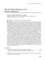
and σ is the Stefan-Boltzmann constant. The actual mean surface temperature
of the Earth is close to 288 K. The effective temperature of emission occurs in
the mid-troposphere, about 5 km above the surface on average. We refer to this
height as Z
e
. As pictured in Figure 1, one can think of the average infrared photon
escaping to space as originating near this mid-tropospheric level. Most photons
P1: FXZ
October 16, 2000 13:0 Annual Reviews AR118-13
WATER VAPOR/GLOBAL WARMING 447
T
s
Tropopause
T
s
+ ∆T
s
Temperature
Altitude
T
e
Z

e
Z
e
+ ∆Z
e
1xCO
2
2xCO
2
Figure 1 Schematic illustration of the change in emission level (Z
e
) associated with an
increase in surface temperature (T
s
) due to a doubling of CO
2
assuming a fixed atmospheric
lapse rate. Note that the effective emission temperature (T
e
) remains unchanged.
emitted from lower in the atmosphere, including most of those emitted from the
surface, are absorbed by infrared-active gases or clouds and are unable to escape
directly to space. The surface temperature is then simply T
s
= T
e
+ Z
e
, where
 is the lapse rate. From this simple perspective, it is the changes in Z

e
, as well
as in the absorbed solar flux and possibly in , that we need to predict when we
perturb the climate. As infrared absorbers increase in concentration, Z
e
increases,
and T
s
increases proportionally if  and S remain unchanged.
The increase in opacity due to a doubling of CO
2
causes Z
e
to rise by ≈150
meters. This results in a reduction in the effective temperature of the emission
across the tropopause by ≈(6.5K/km) (150 m) ≈1 K, which converts to 4W/m
2
using the Stefan-Boltzmann law. This radiative flux perturbation is proportional to
the logarithm of the CO
2
concentration over the range of CO
2
levels of relevance
to the global warming problem. Temperatures must increase by ≈1 K to bring the
system back to an equilibrium between the absorbed solar flux and the infrared flux
escaping th space (Figure 1). In radiative-convective models with fixed relative
humidity, the increase in water vapor causes the effective level of emission to move
upwards by an additional ≈100m for a doubling of CO
2
. Water vapor also absorbs

solar radiation in the near infrared, which feeds back with the same sign as the
P1: FXZ
October 16, 2000 13:0 Annual Reviews AR118-13
448 HELD

SODEN
terrestrial radiation component, accounting for ≈15% of the water vapor feedback
in climate models (20, 21).
In equilibrium, there is a balance between the absorbed solar flux S and the
outgoing terrestrial radiation R. Listing a few of the parameters on which these
fluxes depend, we have, schematically,
S(H
2
O, I, C) = R(T, H
2
O, log
2
CO
2
, C), 1.
where Crepresents clouds, I the ice andsnowcover, log
2
CO
2
is thelogarithm of the
CO
2
concentration (base 2) and T is either the mean surface temperature or a mean
tropospheric temperature (we are assuming here that these temperatures all change
uniformly). Perturbing CO

2
and holding H
2
O, I, and C fixed, the perturbation in
temperature dT satisfies
0 =
∂R
∂T
dT +
∂R
∂log
2
CO
2
dlog
2
CO
2
2.
Linearizing about the present climate, we can summarize the preceding discussion
by setting
∂R
∂T
≈ 4W/(m
2
K) 3.
and
∂ R
∂log
2

CO
2
≈−4W/m
2
4.
so that
dT
dlog
2
CO
2
=−
∂R
∂log
2
CO
2

∂ R
∂ T
≡ 
0
≈ 1K 5.
for fixed H
2
O, C, and I.
If we believe that changes in water vapor are constrained by changes in at-
mospheric temperature, we can set H
2
O = H

2
O(T ). Replacing equation 2, we
have
∂ S
∂ H
2
O
dH
2
O
dT
dT =
∂R
∂T
dT +
∂R
∂H
2
O
dH
2
O
dT
dT +
∂R
∂log
2
CO
2
dlog

2
CO
2
6.
The temperature response to CO
2
doubling is now
dT
dlog
2
CO
2
=

0
1−β
H
2
O
, 7.
where
β
H
2
O
≡

−
∂ R
∂ H

2
O
+
∂ S
∂ H
2
O

dH
2
O
dT

∂R
∂T
. 8.
P1: FXZ
October 16, 2000 13:0 Annual Reviews AR118-13
WATER VAPOR/GLOBAL WARMING 449
The size of nondimensional ratio, β
H
2
O
, provides a measure of the strength of
the water vapor feedback. If β
H
2
O
≈ 0.4, water vapor feedback increases the
sensitivity of temperatures to CO

2
by a factor of ≈1.7, assuming that I and C
are fixed.
If the value of β
H
2
O
were larger than unity, the result would be a runaway
greenhouse. The outgoing infrared flux would decrease with increasing tempera-
tures. It is, of course, self-evident that the Earth is not in a runaway configuration.
But it is sobering to realize that it is only after detailed computations with a
realistic model of radiative transfer that we obtain the estimate β
H
2
O
≈ 0.4 (for
fixed relative humidity). There is no simple physical argument of which we are
aware from which one could have concluded beforehand that β
H
2
O
was less than
unity. The value of β
H
2
O
does, in fact, increase as the climate warms if the relative
humidity is fixed. On this basis, one might expect runaway conditions to develop
eventually if the climate warms sufficiently. Although it is difficult to be quanti-
tative, primarily because of uncertainties in cloud prediction, it is clear that this

point is only achieved for temperatures that are far warmer than any relevant for
the global warming debate (22).
The Satellite Era
Given that the earth’s climate is strongly constrained by the balance between the
absorption of solar radiation and emission of terrestrial radiation, space-based
observations of this radiation budget play a centrally important role in climate
studies. These observations first became available in the mid-1960s. After two
decades of progress in satellite instrumentation, a coordinated network of satellites
[the Earth Radiation Budget Experiment (ERBE)] waslaunched in 1984 to provide
comprehensive measurements of the flow of radiative energy at the top of the
atmosphere (23). Over a century after John Tyndal first noted its importance, an
observational assessment of our understanding of the radiative trapping by water
vapor became possible.
When analyzing the satellite measurements, it has proven to be particularly
valuable to focus on the outgoing longwave fluxes when skies are free of clouds,
R
clear
, to highlight the effects of watervapor. Following Raval & Ramanathan (24),
in Figure 2a (see color insert) we use ERBE observations to plot the annual mean
clear sky greenhouse effect, G
clear
≡ R
s
− R
clear
, over the oceans, where R
s
is the
longwave radiation emitted by the surface. (In the infrared, ocean surfaces emit
very nearly as black bodies, so that R

s
is simply σ T
4
s
.) A simple inspection of these
figures reveals several important features regarding the processes that control the
atmospheric greenhouse effect.
The magnitude of greenhouse trapping is largest over the tropics and decreases
steadily as one approaches the poles. Moreover, the distribution of the clear-sky
greenhouse effect closely resembles that of the vertically-integrated atmospheric
water vapor (Figure 2b; see color insert). The thermodynamic regulation of this
column-integrated vapor is evident when comparing this distribution with that of
P1: FXZ
October 16, 2000 13:0 Annual Reviews AR118-13
450 HELD

SODEN
surface temperature (Figure 2c; see color insert). Warmer surface temperatures
are associated with higher water vapor concentrations, which in turn, are associ-
ated with a larger greenhouse effect. Regressing G
clear
versus T
s
over the global
oceans (24, 25), one finds a relationship that is strikingly similar to that obtained
from radiative computations assuming clear sky, fixed lapse rate, and fixed relative
humidity.
Such an analysis suggests the tantalizing possibility that the strength of water
vapor feedback might be determined directly from observations rather than re-
lying upon models. Unfortunately, life is not so simple. The vapor distribution

in Figure 2 is not solely a function of surface temperature. Even if the relative
humidity were fixed, variations in atmospheric temperature do not always follow
surface temperature changes in a simple way. For example, the relationship be-
tween R
clear
and T
s
obtained from geographic variations in mid-latitudes differs
markedly from those obtained from the local seasonal cycle, owing to differences
in the variations in lapse rate; similarly, the relation observed on seasonal time
scales differs markedly from that observed on interannual time scales (26).
More importantly still, the relative humidity distribution is strongly affected by
the atmospheric circulation, with areas of mean ascent moister than areas of mean
subsidence. Over the tropical oceans, in particular, ascent occurs in the regions
of warmest surface temperature, and strong descent occurs in regions where the
surface is only a few degrees cooler. The circulation can be thought of as forced,
in first approximation, by the difference in surface temperature between these two
regions, not by the absolute temperature itself. Let us suppose that the atmosphere
warms uniformly and that the circulation does not change. Schematically, we can
set R = R(T, ω) where ω is the vertical motion. A simple regression of R with T
in the tropics that does not take into account that ω is spatially correlated with T
incorrectly suggests the existence of a “super-greenhouse effect” (27).
One attempt to avoid this circulation dependence is exemplified by Soden (28),
who averaged over the ascending and descending regions of the tropics and used
interannual variations produced by El Ni˜no as the source of variability. Figure 3
shows the evolution of G
clear
averaged over the tropics for a 4-year period contain-
ing the El Ni˜no event in 1988. An increase in tropical-mean greenhouse trapping
of ≈ 2W/m

2
is observed in conjunction with a ≈0.4 K increase in tropical-mean
sea surface temperature. These tropical mean results are the small difference be-
tween larger regional changes that are dominated by the dramatic changes in the
pattern of ascent and descent that occur during El Ni˜no. There is no reason to
believe that global warming will be accompanied by similar circulation changes.
One can conceive of a number of ways in which the regional changes might be
nonlinearly rectified to produce a tropical mean infrared trapping that is different
in El Ni˜no warming and CO
2
-induced warming. Indeed, at face value, the results
in Figure 3 suggest a value of β
H
2
O
much larger than 0.4.
In recent years, efforts along these lines have been redirected away from at-
tempts at obtaining direct empirical estimates of climate sensitivity, and towards
providing a record of variability against which model predictions may be tested.
As an example, Figure 3 also shows the prediction of a climate model (one
P1: FXZ
November 5, 2000 13:36 Annual Reviews AR118-13
WATER VAPOR/GLOBAL WARMING 451
P1: FXZ
October 16, 2000 13:0 Annual Reviews AR118-13
452 HELD

SODEN
constructed at National Oceanic and Atmospheric Administration’s Geophysical
Fluid Dynamics Laboratory), when the observed sea surface temperatures are used

as a surface boundary condition. The model simulates the variations in clear-sky
infrared trapping very well, although studies of longer data sets suggest that the
response of the moisture field, and the ability of climate models to reproduce the
observed response, may differ from one El Ni˜no event to the next (29). One also
finds that the model does less well at simulating the observed variations in the net
outgoing radiation (solar plus terrestrial, including cloudy as well as clear skies),
once again strongly suggesting that the prediction of clouds and their radiative
properties are the central difficulty facing the model, not water vapor.
Empirical studies such as that in Figure 3 do not provide a direct proxy for
CO
2
-included warming. Rather, the degree of similarity between the observed and
modeled response of G
clear
to changes in surface temperature provides a measure
of confidence in the ability of the climate model to accuratelyrepresent the relevant
physicalprocesses involvedin determiningG
clear
, and thereforeto correctlypredict
thewatervaporfeedback thatwouldoccur undervariousglobal warmingscenarios.
Our dependence on models is unavoidable when analyzing a system as complex
as that maintaining our climate.
Climate Models
The idea of predicting the weather by integrating the equations governing the
atmospheric state forward in time was made explicit by V Bjerknes (30) in 1904.
LF Richardson (31) made the first serious, but famously unsuccessful, attempt at
gathering data to provide an initial condition and actually integrating a version of
these equations. At the dawn of the computer age, J von Neumann, J Charney,
and others realized that the resulting computational power would make numerical
weather prediction feasible. The success of this enterprise has been impressive

(32). Predictions of the atmospheric state for up to 10 days in advance continue
to improve, and the meteorological services of the world continue to be prime
customers of the largest supercomputers in existence, as more computer power
translates into better forecasts.
Building on this effort in weather prediction, through the 1960s and 1970s a
parallel effort began toward the development of numerical models of the Earth’s
climate. In climate modeling, the emphasis shifts to the long-term statistics
of the atmospheric (as well as oceanic and cryospheric) state, and the sensi-
tivity of these statistics to perturbations in external parameters, rather than the
short-term evolution from particular initial conditions. Because they are inte-
grated over longer periods, the spatial resolution of climate models is always
lower than that of state-of-the-art weather prediction models. In the past few
years global warming scenarios have typically been generated using atmospheric
models with effective grid sizes of roughly 200–300 kms, with ≈10 vertical lev-
els within the troposphere. An order of magnitude increase in computer power
allows roughly a factor of two decrease in the effective grid size. Climate warming
P1: FXZ
October 16, 2000 13:0 Annual Reviews AR118-13
WATER VAPOR/GLOBAL WARMING 453
scenarios with horizontal atmospheric resolution of 100 km and less will be-
come available in the next few years. Much more ambitious plans are being
laid. For example, the Japanese frontier Research System for Global Change
() has the goal of constructing a global climate model
with 10 km resolution.
There is a large gap between climate sensitivity experiments with compre-
hensive climate models and computations with simple models like the radiative-
convective model. Because of the turbulent character of atmospheric flows, the
complex manner in which the atmosphere is heated (through latent heat release
and by radiative fluxes modified by intricate cloud distributions) as well as the
rather complex boundary condition that the Earth’s surface provides, it has proven

difficult to develop models of an intermediate complexity to fill this gap, and the
continuing existence of the gap colors the sociology of the science of global warm-
ing. Building and analyzing climate models is an enterprise conducted by a small
number of groups with substantial computational resources.
Many processes occur in the atmosphere and oceans on scales smaller than
those resolved by these models. These scales of motion cannot simply be ignored;
rather, the effects of these small scales on larger scales must be approximated
to generate a meaningful climate. Some aspects of this closure problem have
been reasonably successful, whereas others are ad hoc or are based on empirical
relations that may not be adequate for understanding climate change. Skeptics
focus on these limitations. For a balanced view, it is useful to watch an animation
of the output of such a model, starting from an isothermal state of rest with no
water vapor in the atmosphere and then “turning on the sun,” seeing the jet stream
develop and spin offcyclones and anticyclones with statistics that closely resemble
those observed, watching the Southeast Asian monsoon form in the summer, and
in more recent models, seeing El Ni˜no events develop spontaneously in the Pacific
Ocean.
The first results of the sensitivity of such a climate model to an increase in
CO
2
were presented in 1975 by Manabe & Wetherald (33) with an atmosphere-
only model over an idealized surface with no heat capacity, no seasonal cycle,
and with fixed cloud cover. The equilibrium sensitivity of global mean surface
temperature obtained was ≈3 K for a doubling of CO
2
. The model produced
only small changes in relative humidity throughout the troposphere and thereby
provided the first support from such a model for the use of the fixed–relative
humidity assumption in estimates of the strength of water vapor feedback. The
model’s temperature sensitivity was increased over that obtained in the simpler

radiative-convective models primarily because of the positive surface albedo feed-
back, the retreat of highly reflective snow and ice cover near the poles, which
amplifies the warming. (This extra warming is not confined to high latitudes,
as midlatitude cyclones diffuse some of this extra warming to the tropics as
well). The flavor of more recent research on climate sensitivity with global mod-
els can be appreciated by sampling some of the efforts listed in the references
(34–39).
P1: FXZ
October 16, 2000 13:0 Annual Reviews AR118-13
454 HELD

SODEN
As climate models have evolved to include realistic geography, predicted cloud
cover, and interactions with sea ice and ocean circulation, certain robust conclu-
sions have emerged. In particular, all comprehensive climate models of which we
are aware produce increases in water vapor concentrations that are comparable to
those predicted by fixing the relative humidity. Differences in equilibrium sensi-
tivity among different models appear to be due primarily to differences in cloud
prediction schemes and, to some extent, the treatment of sea ice, and only in a mi-
nor way to differing predictions of water vapor distribution. This point was made
very clearly by the intercomparison study of Cess et al (40), in which a variety of
atmospheric models in an idealized setting were subjected to a uniform increase
in surface temperature. The changes in net radiation at the top of the atmosphere
in the clear sky were generally consistent across the different models, and consis-
tent with fixed relative humidity radiative computations. The total-sky (clear plus
cloudy) fluxes were much less consistent across models.
Recently, Hall & Manabe (41) have artificially removed the radiative conse-
quences of increasing water vapor from a full coupled atmosphere-ocean climate
model. The sensitivity of their model is reduced by more than a factor of 3.5. As
described in the following section, this large response can be understood, to a

rough first approximation, by taking into account how water vapor feedback can
interact with other feedbacks.
The Simplest Feedback Analysis
We can take ice/snow albedo feedback into account schematically by assuming
that I in equation 1 is a function of T. We then have instead of equation 7,
dT
dlog
2
CO
2
=

0
1 − β
H
2
O
− β
I
, 9.
where
β
I
≡
∂ S
∂ I
∂ I
∂T

∂ R

∂T
. 10.
Suppose that the strength of the ice/snow albedo feedback has the value of β
I
=
0.2. In the absence of water vapor feedback, albedo feedback of this strength
increases the temperature response to CO
2
doubling from1Kto≈1.25 K. How-
ever, in the presence of water vapor feedback of strength β
H
2
O
= 0.4, albedo feed-
back increases sensitivity from 1.67 K to 2.5 K. The key here is that the water
vapor and ice/snow albedo perturbations feed on each other, with less ice imply-
ing warmer temperatures, implying more water vapor, and so on. The existence
of strong water vapor feedback increases the importance of other temperature-
dependent feedbacks in the system.
Suppose now that we have a variety of models, all with β
H
2
O
≈ 0.4, but
that produce sensitivities from 1.5–4.5 K for doubling of CO
2
, owing to dif-
fering treatments of other temperature-dependent feedbacks (cloud cover as well
as ice and snow). Figure 4 shows the range of sensitivities that would result if β
H

2
O
P1: FXZ
October 16, 2000 13:0 Annual Reviews AR118-13
WATER VAPOR/GLOBAL WARMING 455
Figure 4 The change in surface temperature T
s
for doubled CO
2
as a function of the water
vaporfeedbackparameterβ
H
2
O
.Resultsare shownfor twodifferentscenariosofothertemperature-
dependent feedbacks β
other
that encompass the current range of predictions in T
s
= 1.5– 4.5K
when β
H
2
O
= 0.4.
had a smaller value in these models. If there were no water vapor feedback, the
maximum sensitivity would be close to 1.5 K, which is the minimum sensitivity
for β
H
2

O
= 0.4. The figure also predicts a result roughly consistent with the Hall
and Manabe coupled model in which water vapor feedback alone is suppressed,
given that that model’s sensitivity is greater than 3.5 K for CO
2
doubling.
Because cloud and water vapor feedbacks are obviously related at some level,
they are often confused in popular discussions of global warming. In the current
generation of climate models, water vapor feedback is robustand cloud feedback is
not. A robust water vapor feedback sensitizes the system, making the implications
of the uncertainty in cloud feedbacks of greater consequence.
The total radiative effect of increases in water vapor can be quite dramatic,
depending on the strengths of the other feedbacks in the system. For the remainder
of this review we return our focus to water vapor feedback in isolation, represented
by β
H
2
O
in the preceding discussion.
P1: FXZ
October 16, 2000 13:0 Annual Reviews AR118-13
456 HELD

SODEN
THE CLIMATOLOGICAL RELATIVE HUMIDITY
DISTRIBUTION
The Global Picture
In Arrhenius’ and Chamberlin’s time, discussions of water vapor feedback neces-
sarily took place without knowledge of the climatological distribution of humidity
except near the Earth’s surface. With the advent and continued maintenance of the

remarkable network of twice-daily balloon ascents, designed for weather forecast-
ing after World War II, the climatological water vapor distribution throughout the
troposphere began to be defined with greater clarity. However, the routine mea-
surement of water vapor, especially in the upper troposphere, is inherently more
difficult than that of temperature and winds, owing in part to problems of contam-
ination as instruments pass through the far wetter lower troposphere. [See Elliott
& Gaffen (42) on the difficulties in using the water vapor fields from the weather
balloon, or radiosonde, network for climate studies.] Additionally, there are rela-
tively few radiosonde ascents in the dry subtropical regions of special interest to
the water vapor feedback debate.
Satellites fill this gap nicely, however. By measuring the upwelling radiance in
different spectral bands that are sensitive to absorption by water vapor, one can ob-
tainmeasurements of watervapor concentrations invariousparts ofthe atmosphere
(43). An example of our current remote sensing capabilities is shown in Figure
5 (see color insert), which depicts the distribution of relative humidity averaged
over the upper troposphere. Note the presence of deep convective clouds (white),
detraining cirrus anvils (gray), the convective moistening of adjacent regions of
high relative humidity (red ), and the gradual reduction in relative humidity as air
is expelled from convective towers and is carried towards the subtropics, subsiding
and warmingowingto adiabatic compression along theway, ultimately resulting in
relative humidities <10%. An international network of satellites provides global
observations of water vapor several times a day and has greatly enhanced our
understanding of its distribution and its radiative effects. Although the measure-
ments shown in Figure 5 are limited to cloud-free regions, satellite sensors capable
of penetrating cloud cover also exist, thus enabling observations of water vapor
under nearly all weather conditions. Whereas better observations would allow us
to test models more definitively, the existing radiosonde/satellite database leaves
little room for major surprises concerning the climatological distribution of water
vapor in the troposphere.
Operational weather prediction centers gather water vapor, temperature, and

wind data from all available sensors, including satellites and radiosondes, and
combine these with predictions from previous forecasts to generate their best es-
timate of the current atmospheric state for use as the initial condition for the
next forecast. Figures 6 and 7 show the relative humidity fields generated by
the European Centre for Medium-Range Weather Forecasting, averaged in time
over the month of July 1987. Figure 6 is an average over longitude. Figure 7 is a
horizontal map of the vertical average over the free troposphere, excluding the
P1: FXZ
October 16, 2000 13:0 Annual Reviews AR118-13
WATER VAPOR/GLOBAL WARMING 457
Figure 6 Height-latitude cross sections of the zonal-mean relative humidity for July 1987 as produced by the European Centre
for Medium-Range Weather Forecasts (ECMWF) analysis system (left) and predicted by the GFDL (Geophysical Fluid Dynamics
Laboratory) General Circulation Model (GCM) (right).
P1: FXZ
October 16, 2000 13:0 Annual Reviews AR118-13
458 HELD

SODEN
Figure 7 The geographic distribution of relative humidity, vertically averaged over the free troposphere for July 1987 from
the ECMWF (European Centre for Medium-Range Weather Forecasts) analyses (left) and the GFDL GCM (Geophysical Fluid
Dynamics Laboratory General Circulation Model) (right).
P1: FXZ
October 16, 2000 13:0 Annual Reviews AR118-13
WATER VAPOR/GLOBAL WARMING 459
lowest 2 km. Also shown are the comparable relative humidities from a climate
model in use for global warming and atmospheric dynamics studies in our labora-
tory (34, 44), assuming as a surface boundary condition the observed sea surface
temperatures from the same time period.
The general features of the humidity distribution are similar in both the opera-
tional analyses and the General Circulation Model (GCM). Note the high values of

relative humidity withinthe planetary boundarylayer near thesurface; the interme-
diate values in the free troposphere in midlatitudes, the dryness of the subtropics,
and the high values near the equatorial tropopause. Detailed evaluations of the
GCM climatologies indicate that most models compare favorably with satellite
observations of the vertically-integrated water vapor mass, although there is a ten-
dency in many GCMs to underestimate the water vapor concentrations by about
5% (45, 46).
The Planetary Boundary Layer
Inthe planetaryboundary layer, thelowest1–2 km, strong verticalturbulentmixing
strives to create a layer of uniform mixing ratio, which given the decrease in
temperature with height forces the relative humidity to increase with height. This
mixing results in a layer of maximum cloudiness near the top of this layer, and
dries the air in the immediate vicinity of the surface, reducing the relative humidity
in the lower parts of the boundary layer to ≈80%, on average.
Most of the Earth’s surface is ocean, and evaporation E from the ocean can be
modeled as proportional to the difference between the saturation vapor pressure at
the surface temperature T
*
and the vapor pressure in the atmosphere at some small
convenient reference height (typically taken to be 10 m), where the temperature is
T
a
and the relative humidity is H
a
:
E ≈ C[e
s
(T
∗
) − H

a
e
s
(T
a
)]. 11.
The constant of proportionality C is itself roughly proportional to the wind speeds
at this reference height. We can rewrite this expression as
E ≈ C[e
s
(T
∗
)(1 − H
a
) + H
a
(e
s
(T
∗
) − e
s
(T
a
))]. 12.
The temperature difference T
*
− T
a
is small enough (especially in the tropics,

where E is the largest) that the term proportional to 1 − H
a
is the larger of the two
terms in Equation 12. Suppose the surface and atmosphere both warm by2Kand
the vapor pressure in the atmosphere does not increase. H
a
would decrease from
≈0.8 to ≈0.7, and 1 − H
a
would increase by ≈50%. The surface winds are highly
unlikely to change dramatically enough to compensate for this large effect. The
energy for this increased evaporation would have to come from the net downward
radiation at the surface, which cannot plausibly change by this amount for such a
small temperature change. Onthis aspect of the problem there is little controversy:
Water vapor in the boundary layer will increase as climate warms to prevent the
near-surface relative humidity from decreasing appreciably.
P1: FXZ
October 16, 2000 13:0 Annual Reviews AR118-13
460 HELD

SODEN
The Free Troposphere
It is useful to have in mind an explicit, even if oversimplified, picture of the main-
tenance of subsaturation in the free troposphere in order to appreciate the pat-
terns in Figures 6 and 7 and discuss their sensitivity. Recall first that the water
vapor mixing ratio r is conserved as air parcels are carried by the winds, except
for the sources and sinks of vapor. Assume that an air parcel is brought to satu-
ration whenever it comes within the planetary boundary layer, and that this is the
only source of vapor. Assume also that whenever e rises above e
s

, condensation
immediately reduces e to e
s
and that rain removes all condensate instantaneously
without moistening the underlying atmosphere.
Nowpickalocationwithintheatmosphere, x, withtemperature Tandpressure p.
The mixing ratio at this point, at a particular time, can be computed by examining
the trajectory of the air parcel at this location. Assuming that the parcel is not
saturated, follow this trajectory backwards in time until one encounters the point
at which saturation last occurred. Label the temperature and pressure at this
point T
c
and p
c
. (If the parcel is already saturated, set T
c
= T and p
c
= p.) In
general, this condensation point will occur at lower pressure p
c
< p, where T
c
is
sufficiently cold; an unsaturated parcel has most likely subsided since it was last
saturated. The vapor pressure at this point is e
s
(T
c
). Conserving mixing ratio

along the trajectory, one finds that vapor pressure at the original point x is given by
(p/p
c
)e
s
(T
c
). To compute the time-averaged vapor pressure, one needs to think of
T
c
and p
c
as suitably averaged using the ensemble of trajectories that pass through
x at different times. As climate changes, the degree of subsaturation at x will be
affected by changes in T(x) and in T
c
and p
c
. In practice the changes in p
c
are
not very important, and we can think of e ∝ e
s
(T
c
). It is not difficult to show
that fixing T − T
c
is now practically equivalent to fixing H. Therefore, within this
simple model, the assumption of fixed relative humidity is in practice equivalent to

the assumption that the change in the temperature of last saturation is on average
similar to the temperature change itself.
The most important effects ignored in this picture are those due to transport and
subsequent re-evaporation of the condensed phase. We return to this complication
below.
One can imagine the change in T
c
differing from the change in T for a variety of
reasons. For example, one can imagine that the warming is spatially uniform but
thatthe verticalexcursionsof air parcelsincrease inextent, sothat thetypical parcel
reaching point x last experienced saturation at a higher altitude where the temper-
ature is colder, thereby causing T
c
to increase less than it otherwise would. The
result would be an increase in T − T
c
and a reduction in H. The assumption of fixed
T − T
c
or H can be thought of as a conservative stance in the absence of convincing
demonstrations to the contrary from models of the atmospheric circulation.
Outside of the tropics, poleward of ≈30
◦
, the cyclones and anticyclones exert
primary control on the relative humidity above the boundary layer (47). In these
extratropical circulations, typical trajectories projected onto the latitude-vertical
P1: FXZ
October 16, 2000 13:0 Annual Reviews AR118-13
WATER VAPOR/GLOBAL WARMING 461
Figure 8 A height-latitude schematic of the large-scale atmospheric trajectories involved

in the transport and mixing of moisture within the troposphere.
plane are as shown schematically in Figure 8, with poleward moving air rising and
equatorward moving air descending. The slopes of these trajectories typically take
airfrom theboundary layerin thesubtropics tothe tropopausein subpolarlatitudes.
Relatively dry air is produced by lifting moist subtropical boundary layer air along
these slantwise paths in the warm sectors of extratropical waves, precipitating out
much of this water, and then descending while returning equatorward.
With this picture in mind, there is no reason to expect that relative humidity will
be exactly maintained in this region as the climate warms. Changes in the strength
or paths of the mid-latitude storms, and the associated trajectories of air parcels,
could alter the relation between the local temperature change and the average tem-
perature change at the point of last saturation. However, the scale of these storms
is relatively large and reasonably well simulated in climate models. Changesin the
extratropical circulation predicted by these models, although potentially of conse-
quence for regional weather patterns, are not large enough to substantially modify
the relative humidity of the extratropical atmosphere as a whole. Distortions due
to subgrid scale processes are less worrisome in extratropical latitudes than in the
tropics, and there is less reason to question the generic model prediction of small
changes in relative humidity.
Before turning to the tropics, we pause to explain why the free troposphere in
the tropics is of primary concern in any analysis of water vapor feedback.
RELATIVE IMPORTANCE OF DIFFERENT PARTS OF THE
TROPOSPHERE FOR WATER VAPOR FEEDBACK
Fix attention on a horizontal location at a particular time of year. Given the vertical
profile of temperature, water vapor, and cloud aerosols, and the CO
2
concentration,
wecan compute theoutgoing infraredflux Rusing a radiativemodel. Fixingclouds
P1: FXZ
October 16, 2000 13:0 Annual Reviews AR118-13

462 HELD

SODEN
and CO
2
, and dividing up the atmosphere in the vertical into a number of layers N,
we can think of R as a function of the surface temperature and of the temperature
and the water vapor pressure in each of these layers. We can then linearize around
the values of these temperatures and water vapor pressures in the current climate
to compute the sensitivity of R to each of these values
δ R =
N

k=1

∂ R
∂T
k
δT
k
+
∂ R
∂e
k
δe
k

. 13.
Rather than treat the dependence on surface temperature separately, we assume
that thechange in temperatureat the surfaceis equal tothe change intemperature in

the lowest atmospheric layer, and include the response to the surface temperature
change in ∂R/∂T
k
within the lowest layer.
The vapor pressure change required to maintain fixed relative humidity, H,in
the face of a small temperature change δT is H(de
s
/dT)δT.If(a)His assumed to
be unchanged and if (b) the temperature change is spatially uniform, then
δ R =
N

k=1

Q
k
T
+ Q
k
e

δT, 14.
where
Q
k
T
≡
∂ R
∂T
k

; Q
k
e
≡
∂ R
∂e
k
H
de
s
dT
. 15.
The temperature change that produces a given global and annual mean change
in outgoing infrared radiation δR is
δT =
δ R
M
T
+ M
e
=
δ R/M
T
1 − β
H
2
O
, 16.
where
M

T
≡
N

k=1
Q
k
T
; M
e
≡
N

k=1
Q
k
e
17.
and
β
H
2
O
=−
M
e
M
T
. 18.
The overbar refers to an average over latitude, longitude, and season.

Figure 9 (see color insert) shows a particular estimate of the functions Q
e
and
Q
T
obtained by the authors. We divide the atmosphere into 10 layers of equal mass
in the vertical, use temperature and humidity data from the European Centre for
Medium-Range Weather Forcasting, and cloud data from the International Satel-
lite Cloud Climatology Project (48). We also average over longitude for display
purposes, and show the result for July only. We obtain from these results that
P1: FXZ
October 16, 2000 13:0 Annual Reviews AR118-13
WATER VAPOR/GLOBAL WARMING 463
β
H
2
O
≈ 0.33 owing to infrared effects alone. Solar absorption, not discussed in
detail here, increases this to ≈0.38
ThefunctionQ
T
isstronglyaffectedbythecloud distribution. Where upperlevel
clouds are prevalent, the outgoing infrared radiation is most sensitive to tempe-
ratures at the level of these emitting surfaces, and is relatively insensitive to tem-
peratures deeper in the atmosphere. Where skies are clearer, lower tropospheric
temperatures control the outgoing flux.
The function Q
e
provides one view of the relative importance of different levels
and latitude zones for the strength of the infrared water vapor feedback. If temper-

atures change uniformly and if relative humidities remain unchanged, this figure
tells us how much of the reduction in outgoing radiation is due to the water vapor
in different regions. One sees that the middle and upper troposphere dominates
the feedback under these conditions. This is a critical and at first glance, perhaps,
a surprising result, given the distribution of vapor, which thins very rapidly as one
moves upwards. The centers of water vapor spectral lines are fully saturated under
atmospheric conditions, and the photons emitted from the lower troposphere can
only escape to space if they are emitted from the wings of spectral lines, where
the upper tropospheric absorption is sufficiently weak but where the emission is
correspondingly inefficient. Emission from the upper troposphere occurs closer
to the centers of these lines, where the emission is stronger.
Figure9 showsthat thesubtropical dryzones aresomewhatmore importantthan
the moister zone in the deep tropics for the strength of the fixed relative humidity
water vapor feedback. This feature is a consequence of the presence of clouds. If
clear skies are assumed to exist everywhere, the maximum in this figure shifts to
the moister regions in the tropics.
The question of the relative importance of different regions for water vapor
feedback is a source of some confusion in the literature. In assessing this relative
importance, one approach has been to assume equal fractional perturbations in
mixing ratio (or, equivalently, vapor pressure), as in Shine & Sinha (6):
δe ∝ e. 19.
Alternatively, Spencer & Braswell (49) perturb the relative humidities in different
regions by equal amounts, so that
δe ∝ e
s
, 20.
which weights dry regions more strongly, thereby emphasizing the free tropo-
sphere at the expense of the boundary layer and the subtropics over the tropics,
as compared with Shine & Sinha. With the normalization we have chosen, the
upper troposphere is also weightedmore heavily than in Shine &Sinha because the

assumption of fixed relative humidity for a uniform temperature change requires
δe ∝
e
e
s
de
s
dT
∝
e
T
2
. 21.
P1: FXZ
October 16, 2000 13:0 Annual Reviews AR118-13
464 HELD

SODEN
However, the weight of the subtropics versus the tropics, which have similar
temperatures, is similar to that obtained with Equation 19; the dry subtropics
are weighted much less heavily than in Spencer & Braswell (49).
There is no ambiguity as to how to compute the relative importance of different
regions for water vapor feedback in a model that predicts changes in water vapor
concentrations; the confusion only arises from differing presumptions as to a
plausible model-independent starting point. Our justification for Equation 21 is
only that it better resembles GCM predictions.
Low resolution can make a climate model too diffusive and can result in the dry
regions of the troposphere being too moist. Yet the radiative transfer is such that,
fora giventemperature profile, changesin theabsorptivityareroughly proportional
to changes in the logarithm of the water vapor concentration (24). If the changes

in vapor pressure are proportional to the vapor pressure itself (as in Equations 19
or 21) the impact on sensitivity of such errors in mean humidity is small. Only if
one assumes that the fractional changes in vapor pressure are much larger in dry
than in moist regions, as implied by Equation 20, can one argue that the absence
of very dry regions in a climate model seriously distorts the sensitivity.
An additional source of confusion is that some studies assume clear skies in
the radiative computation. This has the consequence of inappropriately weighting
the lower troposphere, since clouds interfere with the outgoing infrared radiation
emitted by the lower troposphere more frequently than that from the upper tropo-
sphere. If we regenerate Figure 9 (top) assuming clear skies, the maximum values
occur much lower in the troposphere, in the 500–600 millibar (mb) layer.
If temperature changes are uniform and relative humidities remain unchanged
as the climate warms, these results show that the humidity response in the free
troposphere above 800 mb is responsible for almost all of the infrared water vapor
feedback, leaving only 10% to be contributed by the boundary layer. Roughly
55% of the total is due to the tropical free troposphere (30N–30S)(N = North;
S = South), and 35% to the extratropics. Of this tropical contribution, about
two-thirds, 35% of the total, is due to the upper half of the troposphere, from
100–500 mb.
If relative humidity does change and if the temperature changes are not spatially
uniform, one can generalize Equation 16 to read
δT
∗
=
δ R
M
T
+ M
e
=

δ R/M
T
1 − β
H
2
O
, 22.
where now
M
T
≡
N

k=1
Q
k
T
δ
˜
T
k
; M
e
≡
N

k=1
Q
k
e

δ
˜
e
k
δ
˜
T
k
. 23.
δT
*
is the change in mean surface temperature, δ
˜
T is the temperature change
normalized by δT
*
, and δ
˜
e is the vapor pressure change normalized by the vapor
pressure change required to maintain fixed H. The kernels Q
k
T
and Q
k
e
in Figure 9
are unchanged.
P1: FXZ
October 16, 2000 13:0 Annual Reviews AR118-13
WATER VAPOR/GLOBAL WARMING 465

The temperature changes predictedby climate models are not spatially uniform.
A very robust feature across models is the polar amplification of the temperature
signal, which implies that δ
˜
T is larger than unity in high latitudes, thereby en-
hancing the extratropical as opposed to the tropical contribution to water vapor
feedback. Of potentially greater importance, many climate models predict that
warming in the tropics will be larger in the upper troposphere than in the lower
troposphere (50), ultimately because the moist adiabatic lapse rate decreases with
increasing temperature. If this is the case, and if H is fixed, the tropical upper
troposphere becomes even more dominant in its contribution to M
e
. But M
T
also
increases in value, because the outgoing infrared radiation is sensitive to the tem-
perature of the cloud tops [as in Figure 9 (bottom)]. As a result, the value of β
H
2
O
does not increase significantly. In fact, we have found it difficult to raise β
H
2
O
much above 0.4 for any plausible temperature change profiles, with fixed relative
humidity. [We caution the reader that water vapor feedback is often defined with
δ
˜
T ≡ 1inM
T

(21, 51)]. Similarly, estimates of β
H
2
O
are also insensitive to modest
biases in the water vapor climatology that may be present in a climate model. For
example, introducing a dry bias of 5%, which is typical of that found in many
GCMs (45, 46), into the humidity climatology used in Figure 9 results in less than
a 3% bias in the corresponding estimate of β
H
2
O
.
Extending the approach of Hall & Manabe (41), one can artificially remove the
effect of the water vapor perturbations on radiative fluxes in a climate model, but
onlyin oneregionat atime. Schneider etal(52) have recentlypresented an analysis
of this kind, which suggests that extratropical moisture is of greater importance for
climatic sensitivity than is implied by the purely radiative computations leading
to Figure 7. The reasons for this difference are unclear at present.
THE CONTROVERSY CONCERNING WATER
IN THE TROPICAL FREE TROPOSPHERE
The Complexity of the Tropics
When different groups attempt to construct numerical simulations of an incom-
pletely understood complex system, one might hope that intercomparisons of the
sort described by Cess et al (40) would indicate where the major uncertainties lie.
But it is also possible that all models are making similar mistakes. Indeed, it has
been argued that global climate models all err in their treatment of water vapor
in similar ways, particularly in the tropics (53–57). The source of this concern is
the fact that much of the vertical transport of heat, momentum, and moisture in
the tropics occurs on scales of a few kilometers or less, in turbulent eddies gener-

ated by moist convection, scales that are not explicitly resolved in global climate
models.
Figure 10 (see color insert) is a scene from a numerical simulation (58) of a
small part of the tropical atmosphere, with horizontal extent 130 km × 130 km,