Báo cáo khoa học: "A LOGICAL VERSION OF FUNCTIONAL GRAMMAR" potx
Bạn đang xem bản rút gọn của tài liệu. Xem và tải ngay bản đầy đủ của tài liệu tại đây (561.63 KB, 8 trang )
A LOGICAL VERSION OF FUNCTIONAL GRAMMAR
William C. Rounds
University of Michigan
Xerox PARC
Alexis Manaster-Ramer
IBM T.J. Watson Research Center
Wayne State University
I Abstract
Kay's functional-unification grammar notation [5] is
a way of expressing grammars which relies on very few
primitive notions. The primary syntactic structure is the
feature structure,
which can be visualised as a directed
graph with arcs labeled by attributes of a constituent, and
the primary structure-building operation is unification.
In this paper we propose a mathematical formulation of
FUG, using logic to give a precise account of the strings
and the structures defined by any grammar written in
this notation.
2 Introduction
Our basic approach to the problem of syntactic de-
scription is to use logical formulas to put conditions or
constraints on ordering of constituents, ancestor and de-
scendant relations, and feature attribute information in
syntactic structures. The present version of our logic
has predicates specifically designed for these purposes.
A grammar can be considered as just a logical formula,
and the structures satisfying the formula are the syntactic
structures for the sentences of the language. This notion
goes back to DCG's [0], but our formulation is quite dif-
ferent. In particular, it builds on the logic of Kasper and
Rounds [3], a logic intended specifically to describe fea-
ture structures.
The formulation has several new aspects. First, it
introduces the
oriented
feature
structure as
the primary
syntactic structure. One can think of these structures
as parse trees superimposed on directed graphs, although
the general definition allows much more flexibility. In
fact, our notation does away with the parse tree alto-
gether.
A second aspect of the notation is its treatment of
word order. Our logic allows small grammars to define
free-word order languages over large vocabularies in a way
not possible with standard ID/LP rules. It is not clear
whether or not this treatment of word order was intended
by Kay, but the issue naturally arose during the process
of making this model precise. (Joshi [1] has adopted much
the same conventions in tree adjunct grammar.)
A third aspect of our treatment is the use of fixed-
point formulas to introduce recursion into grammars. This
idea is implicit in DCG's, and has been made explicit in
the logics CLFP and ILFP [9]. We give a simple way of
expressing the semantics of these formulas which corre-
sponds closely to the usual notion of grammatical deriva-
tions. There is an interesting use of
type ~ariables
to
describe syntactic categories and/or constructions.
We illustrate the power of the notation by sketching
how the constructions of relational grammar [7] can be
formulated in the logic. To our knowledge, this is the
first attempt to interpret the relational ideas in a fully
mathematical framework. Although relational networks
themselves have been precisely specified, there does not
seem to be a precise statement of how relational deriva-
tions take place. We do not claim that our formalization
is the one intended by Postal and Perlmutter, but we
do claim that our notation shows clearly the relationship
of relational to transformational grammars on one hand,
and to lexical-functional grammars on the other.
Finally, we prove that the satisfiability problem for our
logic is undecidable. This should perhaps be an expected
result, because the proof relies on simulating Turing ma-
chine computations in a grammar, and follows the stan-
dard undecidability arguments. The satisfiability prob-
lem is not quite the same problem as the
aniversal recog-
nition problem,
however, and with mild conditions on
derivations similar to those proposed for LFG [2], the
latter problem should become decidable.
We must leave efficiency questions unexamined in this
paper. The notation has not been implemented. We view
this notation as a temporary one, and anticipate that
many revisions and extensions will be necessary if it is to
be implemented at all. Of course, FUG itself could be
considered as an implementation, but we have added the
word order relations to our logic, which are not explicit
in FUG.
In this paper, which is not full because of space limi-
tations, we will give definitions and examples in Section
3; then will sketch the relational application in Section 4,
and will conclude with the undecidability result and some
final remarks.
3 Definitions and examples
3.1 Oriented f-structures
In this section we will describe the syntactic structures
to which our logical formulas refer. The next subsection
89
obi,e de~.,. ,C
Figure i: A typical DG.
Figure 2: An oriented f-structure for
a4b4c 4.
will give the logic itself. Our intent is to represent not
only feature information, but also information about or-
dering of constituents in a single structure. We begin with
the unordered version, which is the simple DG (directed
graph) structure commonly used for non-disjunctive in-
formation. This is formalized as an acyclic finite automa-
ton, in the manner of Kasper-Rounds [3]. Then we add
two relations on nodes of the DG: ancestor and linear
precedence. The key insight about these relations is that
they are
partial;
nodes of the graph need not participate
in either of the two relations. Pure feature information
about a constituent need not participate in any ordering.
This allows us to model the "cset" and "pattern" infor-
mation of FUG, while allowing structure sharing in the
usual DG representation of features.
We are basically interested in describing structures
like that shown in Figure i.
A formalism appropriate for specifying such DG struc-
tures is that of finite automata theory. A labeled DG can
be regarded as a transition graph for a partially speci-
fied deterministic finite automaton. We will thus use the
ordinary 6 notation for the transition function of the au-
tomaton. Nodes of the graph correspond to states of the
automaton, and the notation 6(q, z) implies that starting
at state(node) q a transition path actually exists in the
graph labeled by the sequence z, to the state 6(q, z).
Let L be a set of arc labels, and A be a set of atomic
feature values. An ( A, L)- automaton is a tuple
.4 = (Q,6,qo, r)
where Q is a finite set of states, q0 is the initial state, L is
the set of labels above, 6 is a partial function from Q x L to
Q, and r is a partial function from terminating states of A
to A. (q is terminating if 6(q, l) is undefined for all l • L.)
We require that ,4 be connected and acyclic. The map r
specifies the atomic feature values at the final nodes of the
DG. (Some of these nodes can have unspecified values, to
be unified in later. This is why r is only partial.) Let F be
the set of terminating states of.A, and let PC.A) be the set
of full paths of,4, namely the set {z • L* : 6(q0, z) • F}.
Now we add the constituent ordering information to
the nodes of the transition graph. Let Z be the termi-
nal vocabulary (the set of all possible words, morphemes,
etc.) Now r can be a partial map from Q to E u A, with
the requirement that if r(q) • A, then q • F. Next,
let a and < be binary relations on Q, the
ancestor
and
precedence
relations. We require a to be reflexive, an-
tisymmetric and transitive; and the relation < must be
irrefiexive and transitive. There is no requirement that
any two nodes must be related by one or the other of these
relations. There is, however, a compatibility constraint
between the two relations:
v(q, r, 8, t) • Q : (q < ~) ^ (q a s) ^ (~ a t) = s < t.
Note: We have required that the precedence and dom-
inance relations be transitive. This is not a necessary
requirement, and is only for elegance in stating condi-
tions like the compatibility constraint. A better formula-
tion of precedence for computational purposes would be
the "immediate precedence" relation, which says that one
constituent precedes another, with no constituents inter-
vening. There is no obstacle to having such a relation in
the logic directly.
Example. Consider the structure in Figure 2. This
graph represents an oriented f-structure arising from a
LFG-style grammar for the language
{anb"c n
I n > I}.
In this example, there is an underlying CFG given by
the following productions:
S
TC
T aTb lab
C cClc.
The arcs labeled with numbers (1,2,3) are analogous
to arcs in the derivation tree of this grammar. The root
node is of "category" S, although we have not represented
this information in the structure. The nodes at the ends
of the arcs 1,2, and 3 are ordered left to right; in our
logic this will be expressed by the formula I < 2 < 3.
The other arcs, labeled by COUNT and #, are feature
90
arcs used to enforce the counting information required by
the language. It is a little difficult in the graph repre-
sentation to indicate the node ordering information and
the ancestor information, so this will wait until the next
section. Incidentally, no claim is made for the linguistic
naturalness of this example!
3.2 A presentation of the logic
We will introduce the logic by continuing the exam-
ple of the previous section. Consider Figure 2. Particu-
lar nodes of this structure will be referenced by the se-
quences of arc labels necessary to reach them from the
root node. These sequences will be called
paths.
Thus
the path 12223 leads to an occurrence of the terminal
symbol b. Then a formula of the form, say, 12 COUNT -
22 COUNT would indicate that these paths lead to the
same node. This is also how we specify linear precedence:
the last b precedes the first c, and this could be indicated
by the formula 12223<22221.
It should already be clear that our formulas will de-
scribe oriented f-structures. We have just illustrated two
kinds of atomic formula in the logic. Compound formulas
will be formed using A (and), and V (or). Additionally,
let I be an arc label. Then an f-structure will satisfy a for-
mula of the form
I :
¢, iff there is an/-transition from the
root node to the root of a substructure satisfying ~b. What
we have not explained yet is how the recursive informa-
tion implicit in the CFG is expressed in our logic. To do
this, we introduce
type variables as
elementary formulas
of the logic. In the example, these are the "category"
variables S, T, and C. The grammar is given as a system
of equations (more properly, equivalences), relating these
variables.
We can now present a logical formula which describes
the language of the previous section.
S where
S ::~
C ::~
V
T ::-"
V
l:TA2:CA(Icount
2count)
A(1
<2) A~b12
(l:cA2:CA(count # 2count) A¢1~)
(i :CA(count ~ end) A ~I)
(I :aA2:TA3:bA(count # 2count)
A (I
< 2)
A
(2 < 3)
A¢1~z)
(l:aA2:b
A (count #
:
end) A (I <
2)
A ~b12),
where ¢I~ is the formula (e a 1) A (e a 2), in which e is
the path of length 0 referring to the initial node of the
f-structure, and where the other ~ formulas are similarly
defined. (The ~b formulas give the required dominance
information.)
In this example, the set L - (1,2, 3, #, count}, the set
E - {a,b,c},
and the set A {end}. Thus the atomic
symbol "end" does not appear as part of any derived
string. It is easy to see how the structure in Figure 2
satisfies this formula. The whole structure must satisfy
the formula S, which is given recursively. Thus the sub-
structure at the end of the 1 arc from the root must satisfy
the clause for T, and so forth.
It should now be clearer why we consider our logic a
logic for functional grammar. Consider the FUG descrip-
tion in Figure 3.
According to [5, page 149], this descril~tion specifies
sentences, verbs, or noun phrases. Let us call such struc-
tures "entities", and give a partial translation of this de-
scription into our logic. Create the type variables
ENT,
S, VERB,
and
NP.
Consider the recursive formula
ENT
where
ENT
::=
S ::
S v NP v VERB
subj : NP A pred : VERB
A(subj < pred)
A((seomp
: none) V
(seomp : S
A(pred <scomp)))
Notice that the category names can be represented as
type variables, and that the categories
NP
and
VERB
are free type variables. Given an assignment of a set of
f-structures to these type variables, the type
ENT
will
become well-specified.
A few other points need to be made concerning this
example. First, our formula does not have any ancestor
information in it, so the dominance relations implicit in
Kay's patterns axe not represented. Second, our word or-
der conventions are not the same as Kay's. For example,
in the pattern
(subj pred ),
it is required that the sub-
ject be the very first constituent in the sentence, and that
nothing intervene between the subject and predicate. To
model this we would need to add the "immediately left of"
predicate, because our < predicate is transitive, and does
not require this property. Next, Kay uses "CAT" arcs to
represent category information, and considers "NP" to be
an atomic value. It would be possible to do this in our
logic as well, and this would perhaps not allow NPs to be
unified with VERBs. However, the type variables would
still be needed, because they are essential for specifying
recursion. Finally, FUG has other devices for special pur-
poses. One is the use of
nonlocai paths,
which are used
at inner levels of description to refer to features of the
"root node" of a DG. Our logic will not treat these, be-
cause in combination with recursion, the description of
the semantics is quite complicated. The full version of
the paper will have the complete semantics.
9]
cat = S
pattern = (subj pred )
i:i: }
I cat
= VERB ]
$corrlp -~. none ]
pattern = ( scomp) ]
• co~p =
[ ~at
= S ]
J
cat = N P ]
cat = VERB ]
Figure 3: Disjunctive specification in FUG.
3.3
The formalism
3.3.1
Syntax
We summarize the formal syntax of our logic. We
postulate a set A of atomic feature names, a set L of
attribute labels, and a set E of terminal symbols (word
entries in a lexicon.) The type variables come from a
set
TVAR
= {X0,Xt }. The following list gives the
syntactical constructions. All but the last four items are
atomic formulas.
1. NIL
2. TOP
3. X, in which
X E TVAR
4. a, in which a E A
5. o', in which o" E E
6. z<v, in which z and v E L"
7. x c~ V,
in
which z and V E
L"
8. [zt x~], in which each z~ E L=
9./:$
10. @^g,
11. ~v,~
12. ~b where [Xt ::= ~bt; X,~ ::= ~,]
Items (1) and (2) are the identically true and false
formulas, respectively. Item (8) is the way we officially
represent path equations. We could as well have used
equations like z = V, where ~ and V E L', but our deft-
nition lets us assert the simultaneous equality of a finite
number of paths without writing out all the pairwise path
equations. Finally, the last item (12) is the way to express
recursion. It will be explained in the next subsection.
Notice, however, that the keyword where is part of the
syntax.
3.3.2
Semantics
The semantics is given with a standard Tarski defini-
tion based on the inductive structure of wffs. Formulae
are satisfied by pairs (.4,p), where ,4 is an oriented f-
structure and p is a mapping from type variables to sets
off-structures, called an environment. This is needed be-
cause free type variables can occur in formulas. Here are
the official clauses in the semantics:
NIL
always;
TOP
never;
x
iff.4
e
p(X);
a iff 7"(q0) = a, where q0 is the initial state
1. (.4, p)
2. (.4,p)
3. (.4,p)
4.
(.4, p)
of ,4;
5.
(A,p)
6. (.4, p)
T. (.4,p)
8. (.4, p)
~, where o" E ~-, iff r(q0) = o';
v < w iff 6(q0, v) < 6(qo, w);
v a w iff 6(qo, v) a ~(qo, w);
[=~ =.] iffVi,j : 6(q0,zl) = ~(qo,xj);
9. (.4,p) ~ l : ~ iff
(.4/l,p) ~ ~,
where
.4/1
is the
automaton .4 started at 6(qo, l);
10. (A, p) ~ ~ ^ ~ iff (A, p) ~ ~ and (A, p) ~
~;
11. (.4,p) ~ ~ V ~b similarly;
12. (.4,p) ~ ~b where [Xt ::= Ot; X, ::= 0n] iff
for some k, (.4, p(~)) ~ ~b, where p(k) is defined
inductively as follows:
• p(°)(xo = 0;
• p(k+~)(Xd = {B I (~,p(~)) [= ,~,},
and where p(k)(X) = p(X) if X # Xi for any i.
We need to explain the semantics of recursion. Our
semantics has two presentations. The above definition is
shorter to state, hut it is not as intuitive as a syntactic,
operational definition. In fact, our notation
~b where [Xt ::= ~bl Xn ::- ~bn]
92
is meant to suggest that the Xs can be replaced by the Cs
in ¢. Of course, the Cs may contain free occurrences of
certain X variables, so we need to do this same replace-
ment process in the system of Cs beforehand. It turns
out that the replacement process is the same as the pro-
cess of carrying out grammatical derivations, but making
replacements of nonterminal symbols all at once.
With this idea in mind, we can turn to the definition
of replacement. Here is another advantage of our logic -
replacement is nothing more than substitution of formu-
las for type variables. Thus, if a formula 0 has distinct
free type variables in the set D = {Xt An}, and
Ct, , ¢, are formulas, then the notation
denotes the simultaneous replacement of any free occur-
rences of the Xj in 0 with the formula Cj, taking care
to avoid variable clashes in the usual way (ordinarily this
will not be a problem.)
Now consider the formula
¢ where [Xt ::= Ct; X, ::= ¢,].
The semantics of this can be explained as follows. Let
D =
{XI X,~}, and for each k _> 0 define a set of
formulas {¢~k) [ I _< i _< n}. This is done inductively on
k:
~o)
= ¢,[X * TOP : X E
D];
¢(k+1)
elk)
i = ~'i[X : X e O].
These formulas, which can be calculated iteratively, cor-
respond to the derivation process.
Next, we consider the formula ¢. In most grammars,
¢ will just be a "distinguished" type variable, say S. If
(`4, p) is a pair consisting of an automaton and an envi-
ronment, then we define
(`4, p) ~ ¢ where [Xt ::= ¢i; X,t ::= ¢,]
iff for some k,
(.4, p) ~ ¢[X, ,- elk): X, E D].
Example. Consider the formula (derived from a reg-
ular
grammar)
S
where
T "'~
(I :aA2 : S) V(I :hA2 :T) Vc
(I :bA2 : S) V(I :aA2 : T) Vd.
Then, using the above substitutions, and simplifying ac-
cording to the laws of Kasper-Rounds, we have
¢(s o)
C,
¢~) = d;
CH)
=
(1:aA2:c) V(1:bA2:d)Vc;
¢(~)
=
(1:bA2:c) V(1:aA2:d)Vd;
¢(2) = I:aA2:(I:aA2:c) V(I:bA2:d)Vc)
V l:bA2:((l:bA2:c) V(l:aA2:d)Vd)
VC.
The f-structures defined by the successive formulas for S
correspond in a natural way to the derivation trees of the
grammar underlying the example.
Next, we need to relate the official semantics to the
derivational semantics just explained. This is done with
the help of the following lemmas.
Lemma 1 (`4,p) ~ ¢~) ~ (`4, p(k)) ~ ¢i.
Lemma 2 (`4,p) ~ 0[Xj ¢./ : X./ E D]
iff(`4,p')
O, where p°(Xi) = {B ] (B,p) ~ ¢i}, if Xi E D, and
otherwise is p(X).
The proofs are omitted.
Finally, we must explain the notion of the
language
defined by ¢, where ¢ is a logical formula. Suppose for
simplicity that $ has no free type variables. Then the
notion
A ~ 0 makes
sense, and we say that
a
string
w E L(~b) iff for some
subsumpfion.minirnal
f-structure
,4, A ~ ¢, and w is compatible with ,4. The notion
of subsumption is explained in [8]. Briefly, we have the
following definition.
Let ,4 and B be two automata. We say ,4 _ B (.4
subsumes B; B extends `4) iff there is a
homomorphisrn
from `4 to B; that is, a map h : Q.4 Qs such that (for
all existing transitions)
1. h(6.~(q, l)) = 6B(h(q),
l);
2. r(h(q)) = r(q)
for all q such that r(q) E A;
3. h(qoa) = qo~.
It can be shown that subsurnption is a partial order on
isomorphism classes of automata (without orderings), and
that for any formula 4} without recursion or ordering, that
there are a finite number of subsumption-minimal au-
tomata satisfying it. We Consider as candidate structures
for the language defined by a formula, only automata
which are minimal in this sense. The reason we do this
is to exclude f-structures which contain terminal symbols
not mentioned in a formula. For example, the formula
NIL is
satisfied by any f-structure, but only the mini-
mal one, the one-node automaton, should be the principal
structure defined by this formula.
By compatibility we mean the following. In an f-
structure `4, restrict the ordering < to the terminal sym-
bois of,4. This ordering need not be total; it may in fact
be empty. If there is an extension of this partial order on
the terminal nodes to a total order such that the labeling
93
symbols agree with the symbols labeling the positions of
w, then w is compatible with A.
This is our new way of dealing with free word order.
Suppose that no precedence relations are specified in a
formula. Then, minimal satisfying f-structures will have
an empty < relation. This implies that any permutation
of the terminal symbols in such a structure will be al-
lowed. Many other ways of defining word order can also
be expressed in this Logic, which enjoys an advantage over
ID/LP rules in this respect.
4 Modeling Relational Grammar
Consider the relational analyses in Figures 4 and 5.
These analyses, taken from [7], have much in common
with functional analyses and also with transsformational
ones. The present pair of networks illustrates a kind of
raising construction common in the relational literature.
In Figure 4, there are arc labels P, I, and 2, representing
"predicate", "subject", and "object" relations. The "cl"
indicates that this analysis is at the first linguistic stra-
tum,
roughly like a transformational cycle. In Figure 5,
we learn that at the second stratum, the predicate ("be-
lieved") is the same as at stratum i, as is the subject.
However, the object at level 2 is now "John", and the
phrase "John killed the farmer" has become a "chSmeur"
for level 2.
The relational network is almost itself a feature struc-
ture. To make it one, we employ the trick of introducing
an arc labeled with l, standing for "previous level". The
conditions relating the two levels can easily be stated as
path equations, as in Figure 6.
The dotted lines in Figure 6 indicate that the nodes
they connect are actually identical. We can now indicate
precisely other information which might be specified in
a
relational
grammar,
such as the ordering information
I < P < 2. This would apply to the "top level", which
for Perlmutter and Postal would be the "final level", or
surface level. A recursive specification would also become
possible: thus
SENT ::= CLAUSEA(I<P<2)
CLAUSE ::= I:NOMAP:VERB
A 2 : (CLAUSE V NOM)
A (RAISE V PASSIVE V )
A I : CLAUSE
l : 2 : CLAUSE A (equations in (6)) RAISE ::=
This is obviously an incomplete grammar, but we think
it possible to use this notation to give a complete specifi-
cation of an RG and, perhaps at some stage, a computa-
tional test.
5 Undecidability
In this section we show that the problem of
sa(is/ia-
bility -
given a formula, decide if there is an f-structure
satisfying it - is undecidable. We do this by building a for-
mula which describes the computations of a given Turing
machine. In fact, we show how to speak about the com-
putations of an automaton with one stack (a pushdown
automaton.) This is done for convenience; although the
halting problem for one-stack automata is decidable, it
will be clear from the construction that the computation
of a two-stack machine could be simulated as well. This
model is equivalent to a Turing machine - one stack rep-
resents the tape contents to the left of the TM head, and
the other, the tape contents to the right. We need not
simulate moves which read input, because we imagine the
TM started with blank tape. The halting problem for
such machines is still undecidable.
We make the following conventions about our PDA.
Moves are of two kinds:
• qi : push b; go to qj ;
• qi : pop stack; if a go to qj else go to
qk.
The machine has a two-character stack alphabet {a, b}.
(In the push instruction, of course pushing "a" is allowed.)
If the machine attempts to pop an empty stack, it can-
not continue. There is one final state qf. The machine
halts sucessfully in this and only this state. We reduce
the halting problem for this machine to the satisfiability
problem for our logic.
Atoms:
"none bookkeeping marker
for
telling what
is in the
stack
qO, ql qn one for
each state
Labels:
a, b for describing
stack contents
s pointer to top of stack
next
value
of next
state
p pointer to previous
stack configuration
Type
variables:
CONF
structure represents
a machine configuration
INIT0 FINAL confi~trations
at start and finish
QO QN: property of being
in
one of these states
The simulation proceeds as in the relational grammar
example. Each configuration of the stack corresponds to
a level in an RG derivation. Initially, the stack is empty.
Thus we put
94
Figure 4: Network for The woman believed that John killed the farmer.
b~ p c a.
f
Figure 5: Network for The woman believed John to have killed the farmer.
p = lp
1 = ll
2 = 121
Chop = 12P
Cho 2 " 1 2 2
Figure 6: Representing Figure 5 as an f-structure.
95
INIT
::= s : (b : none A a : none) A nerl; : q0.
Then we describe standard configurations:
C0//F ::=
ISIT
V (p : CONF A (QO V V QN)).
Next, we show how configurations are updated, de-
pending on the move rules. If q£ is push b; go to qj, then
we write
QI ::=nex~:qjAp:next:qiAs:a:noneAsb=ps.
The last clause tells us that the current stack contents,
after finding a %" on top, is the same as the previous
contents. The %: none" clause guarantees that only a
%" is found on the DG representing the stack. The sec-
ond clause enforces a consistent state transition from the
previous configuration, and the first clause says what the
next state should be.
If q£ is
pop
stack; if a go to qj else go to qk,
then we write the following.
QI
::= p : nex~ : qi
A ((s=psaAnex~::qjAp:s:b:none)
V(s=psbAnext:qkAp:s:a:none))
For the last configuration, we put
I~F
::
C011F
A
p
: nex~ :
qf.
We take QF as the "distinguished predicate" of our
scheme.
It should be clear that this formula, which is a big
where-formula, is satisfiable if[" the machine reaches state
qf.
6 Conclusion
It would be desirable to use the notation provided
by our logic to state substantive principles of particu-
lax linguistic theories. Consider, for example, Kashket's
parser for Warlpiri [4], which is based on GB theory. For
languages like Warlpiri, we might be able to say that
linear order is only explicitly represented at the mor-
phemic level, and not at the phrase level. This would
translate into a constraint on the kinds of logical for-
mulas we could use to describe such languages: the <
relation could only be used as a relation between nodes
of the
MORPHEME
type. Given such a condition on
formulas, it migh t then be possible to prove complexity
results which were more positive than a general undecid-
ability theorem. Similar remarks hold for theories like
relational grammar, in which many such constraints have
been studied. We hope that logical tools will provide a
way to classify these empirically motivated conditions.
References
[1] Joshi, A. , K. Vijay-Shanker, and D. Weir, The Con-
vergence of Mildly Context-Sensitive Grammar For-
malisms. To appear in T. Wasow and P. Sells, ed.
"The Processing of Linguistic Structure", MIT Press.
[2] Kaplan, R. and J. Bresnan, LFG: a Formal Sys-
tem for Grammatical Representation, in Bresnan,
ed. The Mental Representation of Grammatical Re-
lations, MIT Press, Cambridge, 1982, 173-281.
[3] Kasper, R. and W. Rounds, A Logical Semantics for
Feature Structures, Proceedings of e4th A CL Annual
Meeting, June 1986.
[4] Kashket, M. Parsing a free word order language:
Warlpiri. Proc. 24th Ann. Meeting of ACL, 1986,
60-66.
[5] Kay, M. Functional Grammar. In Proceedings of the
Fifth Annual Meeting of the Berkeley Linguistics So-
ciety, Berkeley Linguistics Society, Berkeley, Califor-
nia, February 17-19, 1979.
[6] Pereira, F.C.N., and D. Warren, Definite Clause Gram-
mars for Language Analysis: A Survey of the Formal-
ism and a Comparison with Augmented Transition
Networks, Artificial Intelligence 13, (1980), 231-278.
[7] Perlmutter, D. M., Relational Grammar, in Syntax
and Semantics, voi. 18: Current Approaches to Syn-
taz, Academic Press, 1980.
[8] Rounds, W. C. and R. Kasper. A Complete Logi-
cal Calculus for Record Structures Representing Lin-
guistic Information. IEEE Symposium on Logic in
Computer Science, June, 1986.
[9] Rounds, W., LFP: A Formalism for Linguistic De-
scriptions and an Analysis of its Complexity, Com-
putational Linguistics, to appear.
96